Standard analysis workflow for PBMCs (5,000 cells)
The scRNA-seq data can be downloaded from http://cf.10xgenomics.com/samples/cell-exp/3.0.2/5k_pbmc_v3/5k_pbmc_v3_filtered_feature_bc_matrix.tar.gz
We use SingCellaR to read in matrices found in the “filtered_feature_bc_matrix” folder, which was generated by Cell Ranger software from 10x Genomics. The ‘load_matrices_from_cellranger’ function reads in the output folder and return SingCellaR object.
SingCellaR object initialization
First, SingCellaR will be loaded into R.
library(SingCellaR)

data_matrices_dir<-"../SingCellaR_example_datasets/10x_genomics_5K_PBMCs/filtered_feature_bc_matrix/"
PBMCs<-new("SingCellaR")
PBMCs@dir_path_10x_matrix<-data_matrices_dir
PBMCs@sample_uniq_id<-"PBMCs"

load_matrices_from_cellranger(PBMCs,cellranger.version = 3)
## [1] "The sparse matrix is created."PBMCs## An object of class SingCellaR with a matrix of : 33538 genes across 5025 samples.Cell information will be processed. The “mito_genes_start_with” is an important parameter. The percentage of mitochondrial reads per cell will be calculated. For human, mitochondrial gene names start with “MT-”.
process_cells_annotation(PBMCs,mito_genes_start_with ="MT-")## [1] "List of mitochondrial genes:"
## [1] "MT-ND1" "MT-ND2" "MT-CO1" "MT-CO2" "MT-ATP8" "MT-ATP6" "MT-CO3"
## [8] "MT-ND3" "MT-ND4L" "MT-ND4" "MT-ND5" "MT-ND6" "MT-CYB"
## [1] "The meta data is processed."QC plots
Histogram
plot_cells_annotation(PBMCs,type="histogram")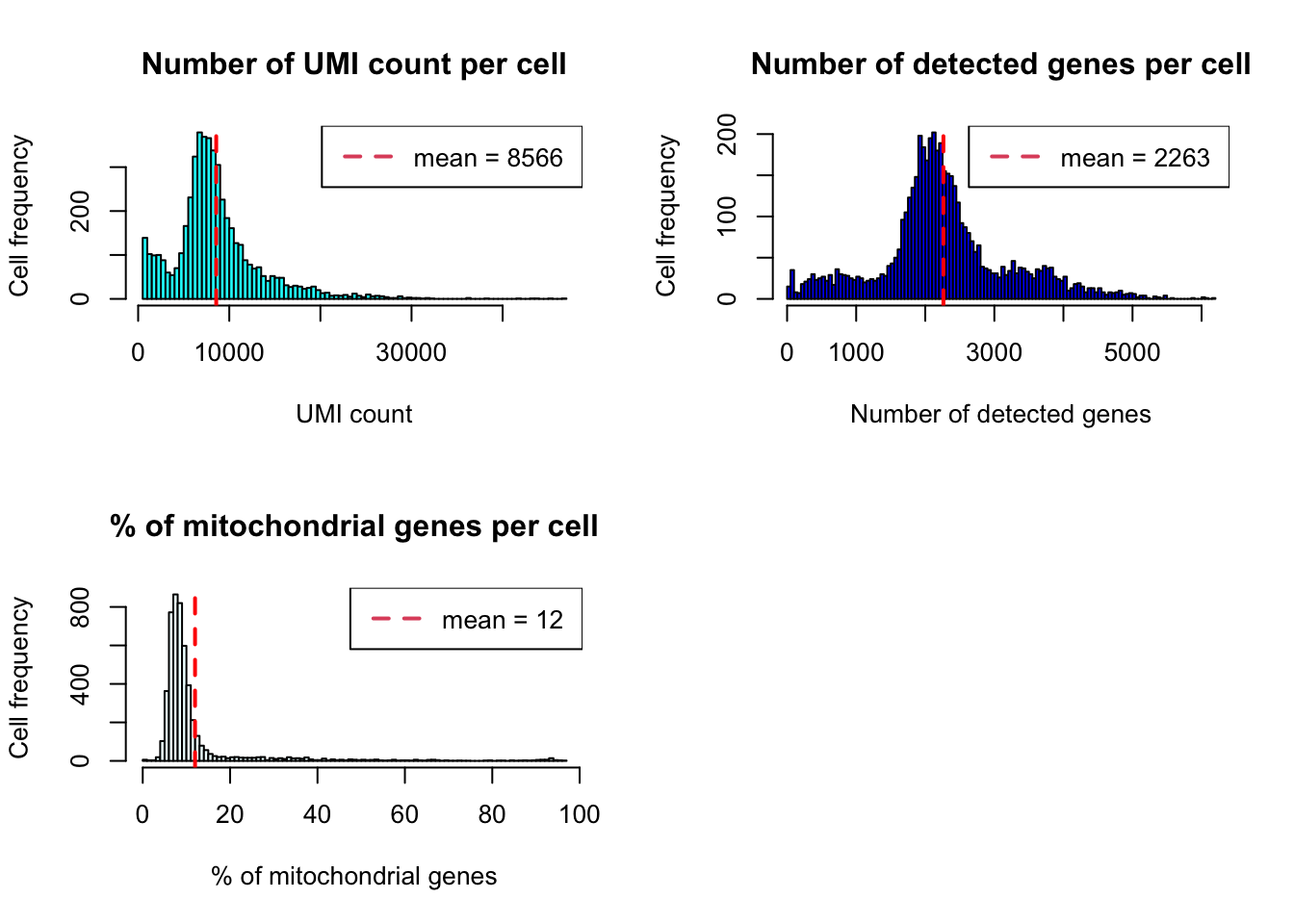
Boxplot
plot_cells_annotation(PBMCs,type="boxplot")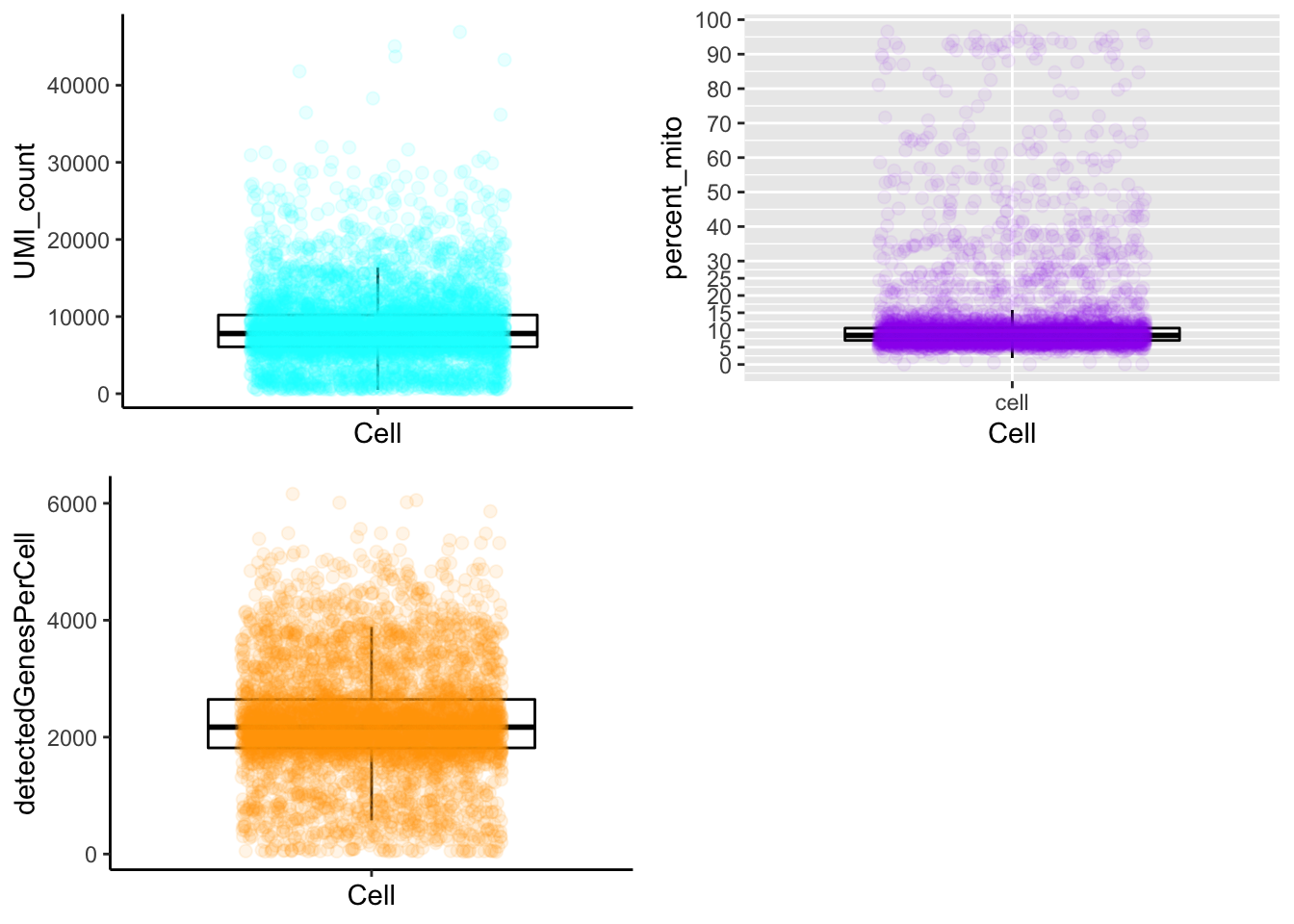
UMI counts/cell vs. detected genes/cell
plot_UMIs_vs_Detected_genes(PBMCs)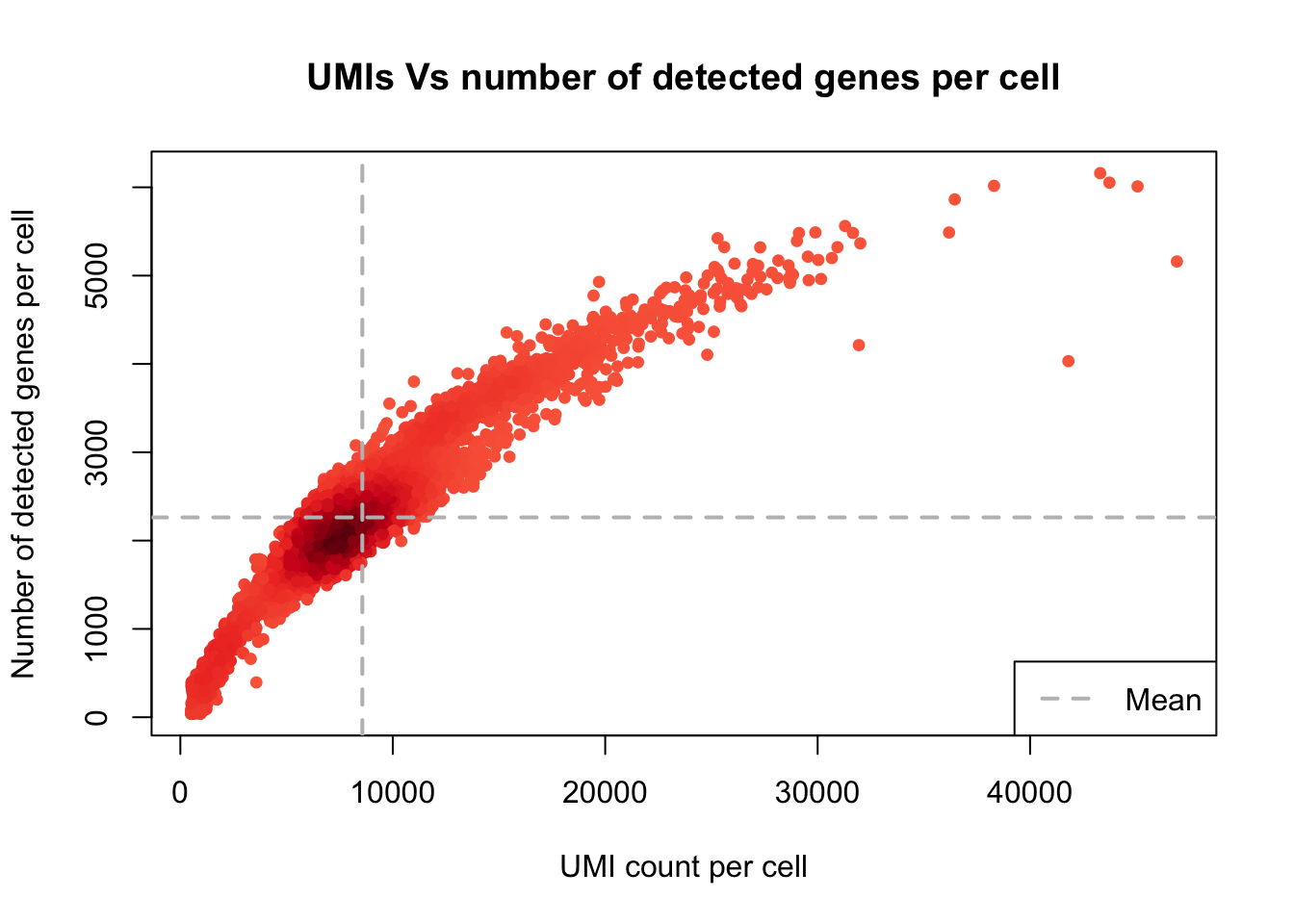
- min_UMIs=1000
- max_UMIs=30000
- min_detected_genes=500
- max_detected_genes=5000
- max_percent_mito=15
- genes_with_expressing_cells=10
Filtering
filter_cells_and_genes(PBMCs,
                       min_UMIs=1000,
                       max_UMIs=30000,
                       min_detected_genes=300,
                       max_detected_genes=5000,
                       max_percent_mito=15,
                       genes_with_expressing_cells = 10,isRemovedDoublets = FALSE)
## [1] "The cells and genes metadata are updated by adding the filtering status."
## [1] "652/5025 cells will be filtered out from the downstream analyses!."Optional: We have incorporated the Scrublet (Wolock et al., 2019) for doublet removal into the latest version of SingCellaR. The user can add the optional step below to detect and exclude doublets:
DoubletDetection_with_scrublet(PBMCs)## [1] "Processing Scrublet.."
## [1] "Doublet prediction result is added in the metadata."table(PBMCs@meta.data$Scrublet_type)##
## Doublets Singlet
## 96 4929Remove doublets
Now, the users can set ‘isRemovedDoublets = TRUE’ to remove potential doublets.
filter_cells_and_genes(PBMCs,
                       min_UMIs=1000,
                       max_UMIs=30000,
                       min_detected_genes=300,
                       max_detected_genes=5000,
                       max_percent_mito=15,
                       genes_with_expressing_cells = 10,isRemovedDoublets = TRUE)
## [1] "The cells and genes metadata are updated by adding the filtering status."
## [1] "738/5025 cells will be filtered out from the downstream analyses!."Normalization
If, “use.scaled.factor=T”, this will scale UMI counts by normalizing each library size to 10000. If, FALSE, this will be scaled to the average number of library sizes.
normalize_UMIs(PBMCs,use.scaled.factor = T)## [1] "Normalization is completed!."Regressing source of variations
Next, the effect of the library size and the percentage of mitochondrial reads are regressed out.
remove_unwanted_confounders(PBMCs,residualModelFormulaStr="~UMI_count+percent_mito")##
|
| | 0%
|
|==== | 6%
|
|======== | 12%
|
|============ | 18%
|
|================ | 24%
|
|===================== | 29%
|
|========================= | 35%
|
|============================= | 41%
|
|================================= | 47%
|
|===================================== | 53%
|
|========================================= | 59%
|
|============================================= | 65%
|
|================================================= | 71%
|
|====================================================== | 76%
|
|========================================================== | 82%
|
|============================================================== | 88%
|
|================================================================== | 94%
|
|======================================================================| 100%
## [1] "Removing unwanted sources of variation is done!"Identify variable genes
The function below will use general linear model (GLM) to model coefficient of variance and mean of gene expression, similarly described in Brennecke et al., Nature Method, 2013.
get_variable_genes_by_fitting_GLM_model(PBMCs,mean_expr_cutoff = 0.05,disp_zscore_cutoff = 0.05)## [1] "Calculate row variance.."
##
|
| | 0%
|
|========= | 12%
|
|================== | 25%
|
|========================== | 38%
|
|=================================== | 50%
|
|============================================ | 62%
|
|==================================================== | 75%
|
|============================================================= | 88%
|
|======================================================================| 100%[1] "Using :12521 genes for fitting the GLM model!"
## [1] "Identified :1992 variable genes"House keeping (e.g. ribosomal genes) and mitochondrial genes should be removed from the variable gene set. SingCellaR reads in GMT file that contains ribosomal and mitochondrial genes and removes these genes from the list of variable genes. Below shows how to use the function.
remove_unwanted_genes_from_variable_gene_set(PBMCs,gmt.file = "../SingCellaR_example_datasets//Human_genesets/human.ribosomal-mitocondrial.genes.gmt",
                                             removed_gene_sets=c("Ribosomal_gene","Mitocondrial_gene"))
## [1] "1 genes are removed from the variable gene set."Here, the plot shows highly variable genes (cyan) in the fitted GLM model.
plot_variable_genes(PBMCs)## [1] "Calculate row variance.."
##
|
| | 0%
|
|========= | 12%
|
|================== | 25%
|
|========================== | 38%
|
|=================================== | 50%
|
|============================================ | 62%
|
|==================================================== | 75%
|
|============================================================= | 88%
|
|======================================================================| 100%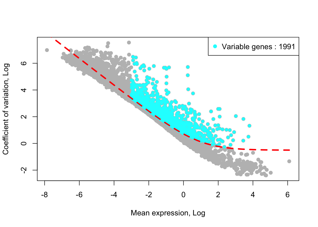
SingCellaR also provides “get_variable_genes_basic”, a simple function for the identification of highly variable genes based on the coefficient of variance and average gene expression.
PCA anlysis
Top 30 PCs will be calculated using the IRLBA method from https://github.com/bwlewis/irlba The parameter “use.regressout.data” is critical. If TRUE, PCA uses the regressed out data. If FALSE, PCA uses the normalized data without removing the unwanted source of variations.
runPCA(PBMCs,use.components=30,use.regressout.data = T)## [1] "PCA analysis is done!."Next, the number of PCs used for downstream analyses will be determined from the scree plot.
plot_PCA_Elbowplot(PBMCs)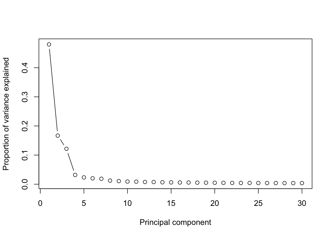
tSNE analysis
Run tSNE analysis with the PCAs.
runTSNE(PBMCs,dim_reduction_method = "pca",n.dims.use = 10)## [1] "TSNE analysis is done!."plot_tsne_label_by_qc(PBMCs,point.size = 0.1)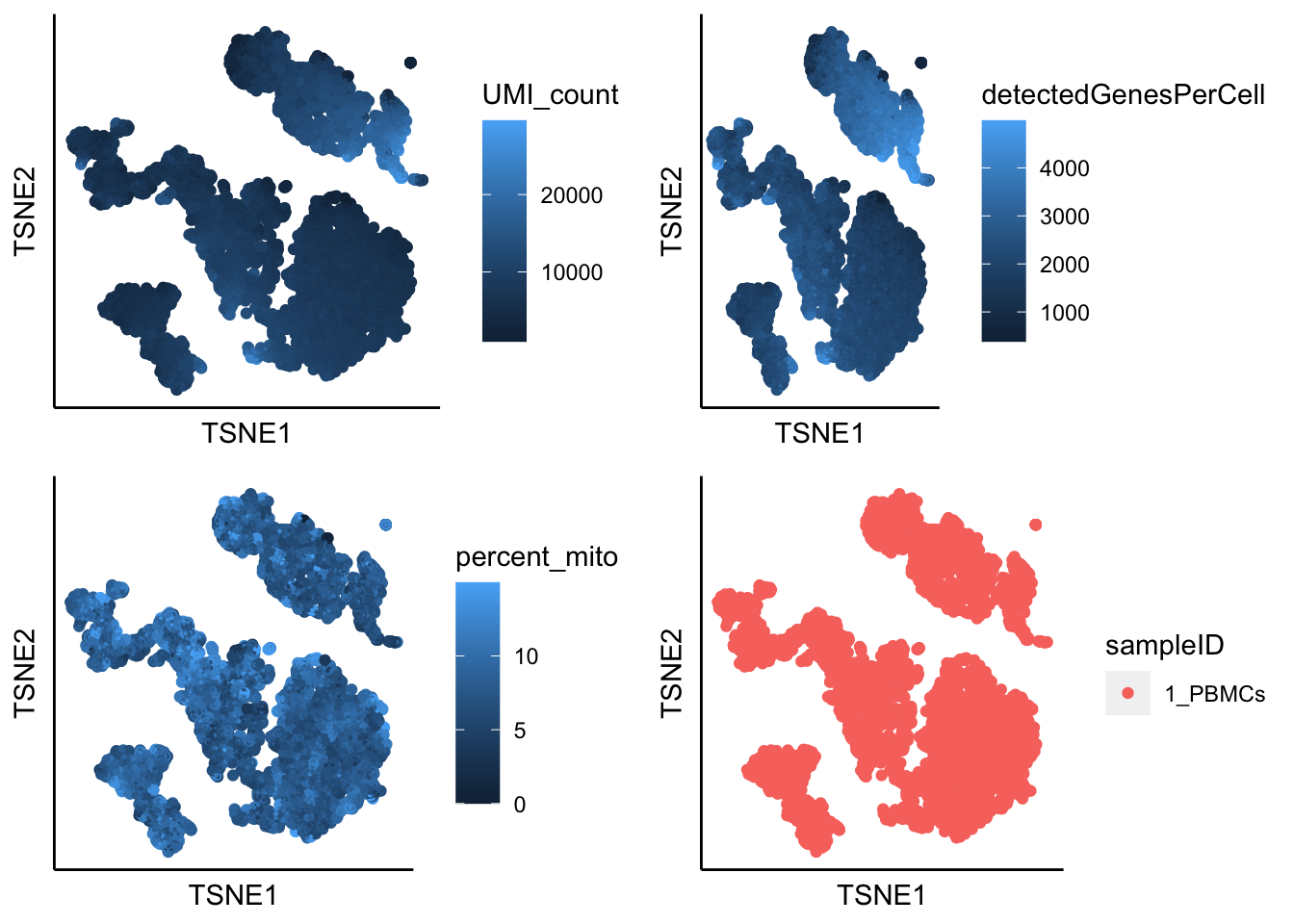
UMAP analysis
runUMAP(PBMCs,dim_reduction_method = "pca",n.dims.use = 10,n.neighbors = 20,
        uwot.metric = "euclidean")
## 16:26:28 UMAP embedding parameters a = 1.121 b = 1.057## 16:26:28 Read 4287 rows and found 10 numeric columns## 16:26:28 Using Annoy for neighbor search, n_neighbors = 20## 16:26:28 Building Annoy index with metric = euclidean, n_trees = 50## 0% 10 20 30 40 50 60 70 80 90 100%## [----|----|----|----|----|----|----|----|----|----|## **************************************************|
## 16:26:29 Writing NN index file to temp file /var/folders/c6/_w309xr54n7cphf9nw4x_ms40000gn/T//Rtmpt059js/fileba9e467cf812
## 16:26:29 Searching Annoy index using 8 threads, search_k = 2000
## 16:26:29 Annoy recall = 100%
## 16:26:29 Commencing smooth kNN distance calibration using 8 threads
## 16:26:30 Found 2 connected components, falling back to 'spca' initialization with init_sdev = 1
## 16:26:30 Initializing from PCA
## 16:26:30 Using 'irlba' for PCA
## 16:26:30 PCA: 2 components explained 72.3% variance
## 16:26:30 Commencing optimization for 500 epochs, with 111964 positive edges
## 16:26:35 Optimization finished## [1] "UMAP analysis is done!."plot_umap_label_by_a_feature_of_interest(PBMCs,feature = "UMI_count",point.size = 0.1,mark.feature = F)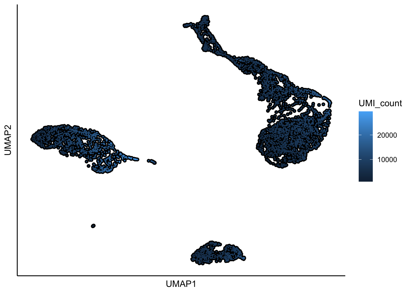
Cluster identification
Cells are clustered based on the K-Nearest Neighbor (KNN) approach, using euclidean or cosine metrice as the input parameter. The weighted graph is created with weight values calculated from normalized shared number of nearest neighbors. The function ‘cluster_louvain’ from the igraph package (Csardi and Nepusz, 2005) is then applied to identify clusters.
Below example shows how to perform clustering analysis.
identifyClusters(PBMCs,n.dims.use = 10,n.neighbors = 100,knn.metric = "euclidean")## [1] "Building Annoy index with metric = euclidean , n_trees = 50"## 0% 10 20 30 40 50 60 70 80 90 100%## [----|----|----|----|----|----|----|----|----|----|## **************************************************|## [1] "Searching Annoy index, search_k = 10000"## 0% 10 20 30 40 50 60 70 80 90 100%
## [----|----|----|----|----|----|----|----|----|----|
## **************************************************|## [1] "Building graph network.."
## [1] "Building graph network is done."
## [1] "Process community detection.."
## [1] "Louvain analysis is done!."Identified clusters are superimposed on top of the tSNE plot.
plot_tsne_label_by_clusters(PBMCs,show_method = "louvain",point.size = 2)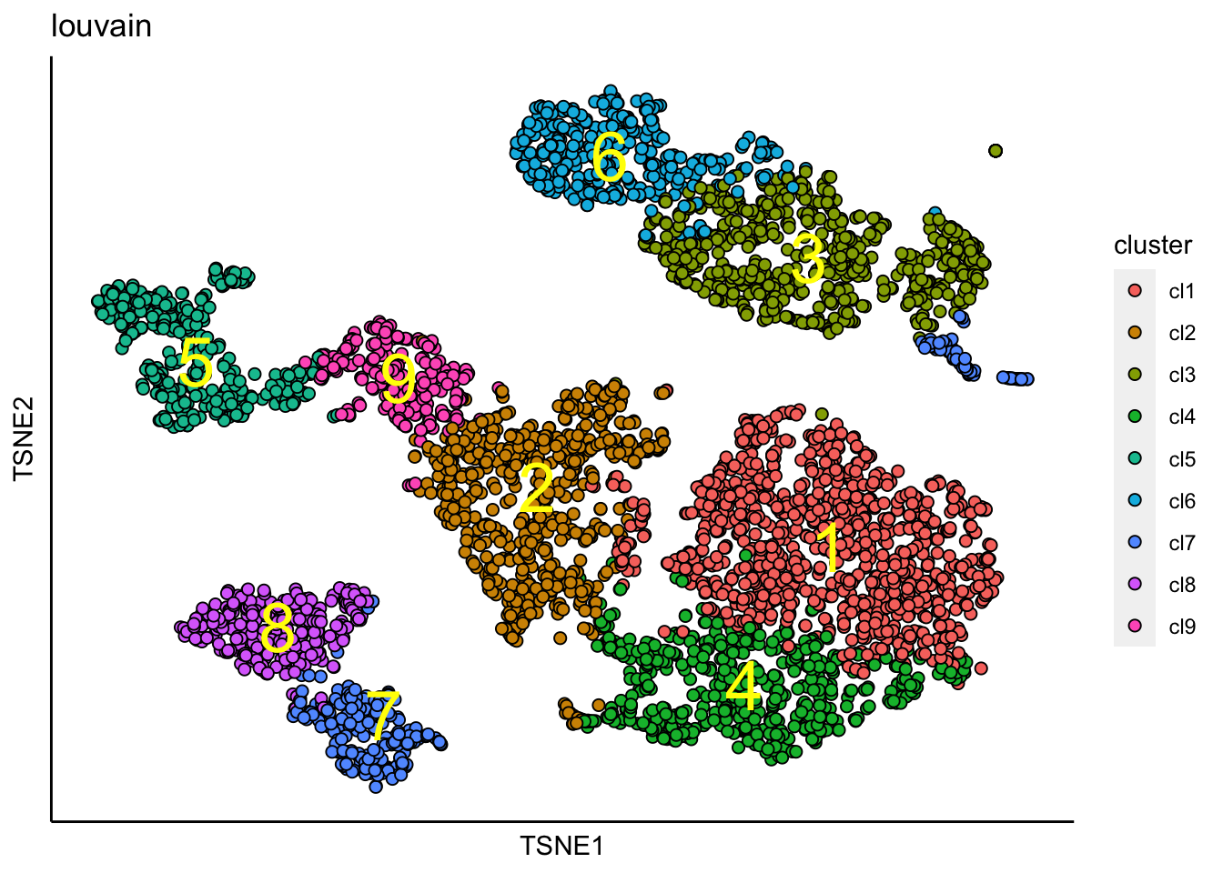
Similary, identified clusters are superimposed on top of the UMAP.
plot_umap_label_by_clusters(PBMCs,show_method = "louvain",point.size = 0.80)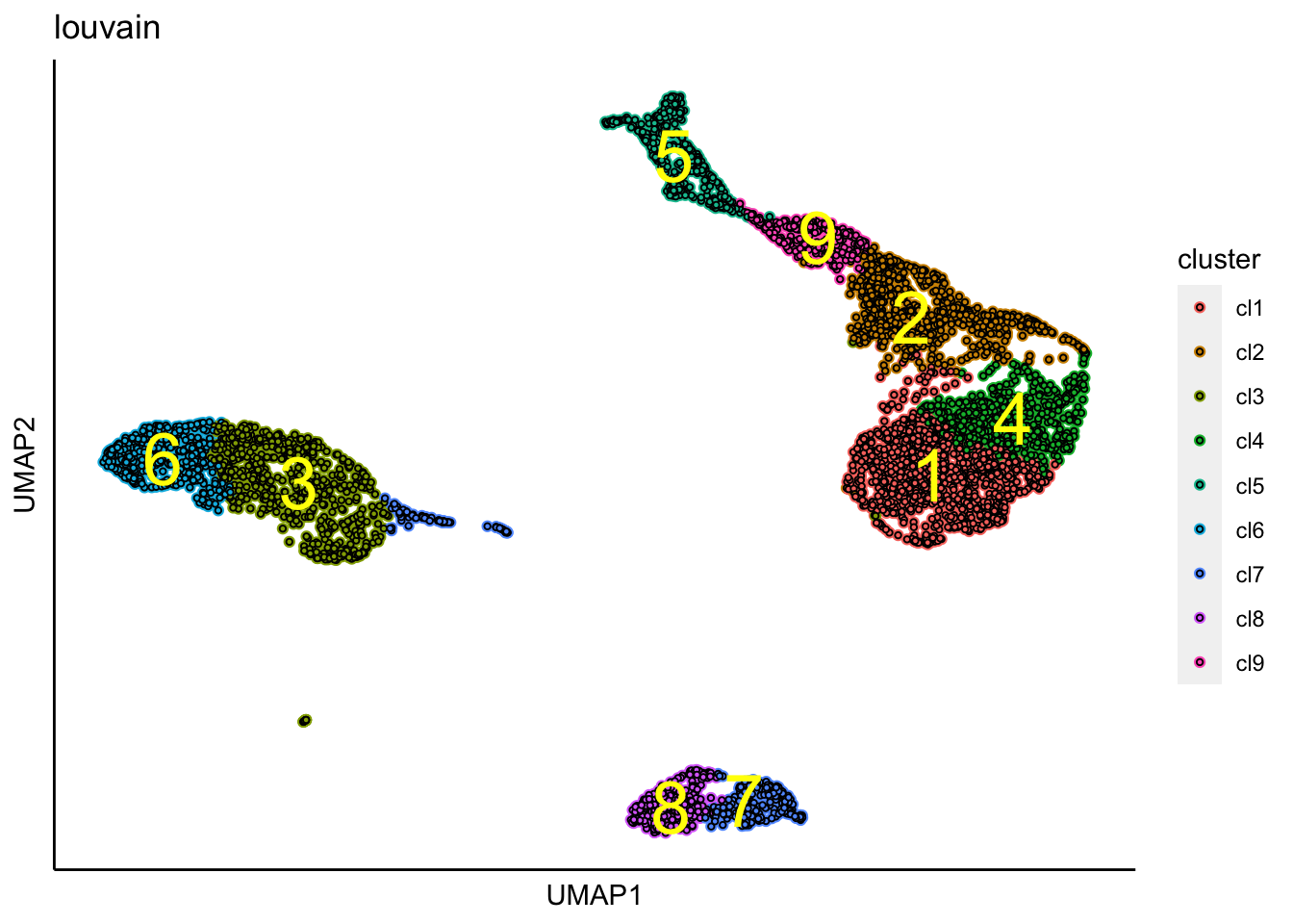
Force-directed graph analysis
SingCellaR incorporates Force-directed graph for the visualization of cellular trajectories. Below is an example to perform Force-directed graph analysis.
runFA2_ForceDirectedGraph(PBMCs,n.dims.use = 10,
                          n.neighbors = 5,n.seed = 1,fa2_n_iter = 1000)
## [1] "Building Annoy index with metric = euclidean , n_trees = 50"## 0% 10 20 30 40 50 60 70 80 90 100%## [----|----|----|----|----|----|----|----|----|----|## **************************************************|## [1] "Searching Annoy index, search_k = 500"## 0% 10 20 30 40 50 60 70 80 90 100%
## [----|----|----|----|----|----|----|----|----|----|
## **************************************************|## [1] "Processing fa2.."
## [1] "Force directed graph analysis is done!."Force-directed graph is then superimposed with identified clusters.
plot_forceDirectedGraph_label_by_clusters(PBMCs,show_method = "louvain",vertex.size = 1,
                                          background.color = "black")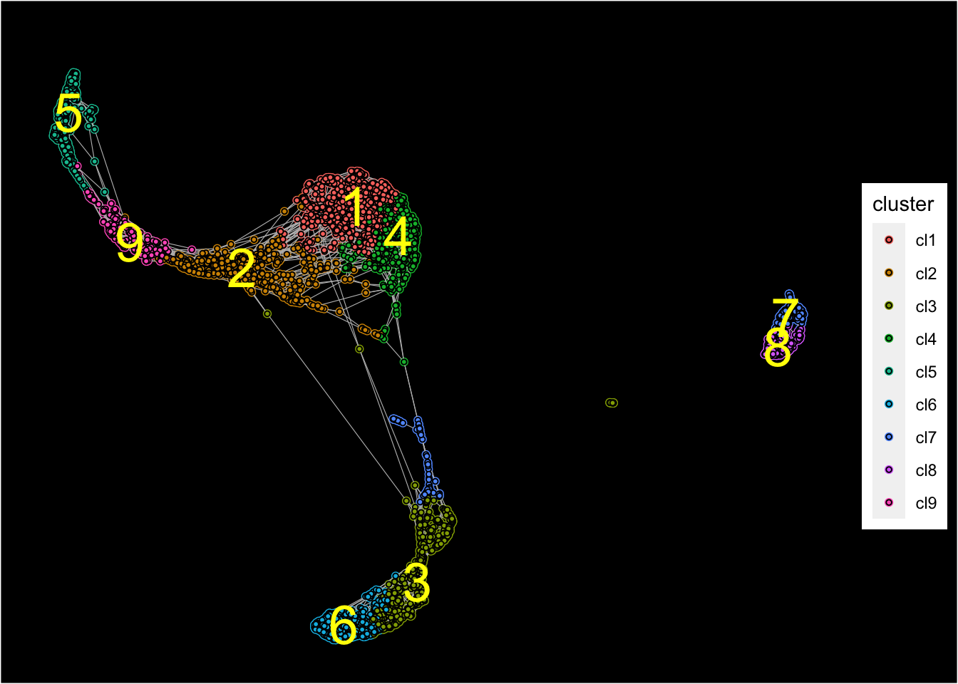
Marker gene identification
Next, differential gene expression analysis will be performed across clusters to identify marker genes that are expressed in each cluster.
SingCellaR combines Wilcoxon test on the log-transformed (normalized UMIs) to compare expression level and Fisher′s exact test to compare the expressing cell frequency of each gene as previously described (Giustacchini et al., Nature Medicine, 2017). P-values generated from both tests are then combined using Fisher’s method and are adjusted using the Benjamini-Hochberg (BH) correction. Genes expressed in each cluster are compared to all other clusters.
findMarkerGenes(PBMCs,cluster.type = "louvain")## [1] "Number of genes for analysis: 15911"
## [1] "Creating binary matrix.."
## [1] "Finding differential genes.."
## [1] "Identifying marker genes for: cl1"
## [1] "Processing Fisher's exact test!"
## [1] "Processing Wilcoxon Rank-sum test!"
## [1] "Combining p-values using the fisher's method!"
## [1] "Identifying marker genes for: cl2"
## [1] "Processing Fisher's exact test!"
## [1] "Processing Wilcoxon Rank-sum test!"
## [1] "Combining p-values using the fisher's method!"
## [1] "Identifying marker genes for: cl3"
## [1] "Processing Fisher's exact test!"
## [1] "Processing Wilcoxon Rank-sum test!"
## [1] "Combining p-values using the fisher's method!"
## [1] "Identifying marker genes for: cl4"
## [1] "Processing Fisher's exact test!"
## [1] "Processing Wilcoxon Rank-sum test!"
## [1] "Combining p-values using the fisher's method!"
## [1] "Identifying marker genes for: cl5"
## [1] "Processing Fisher's exact test!"
## [1] "Processing Wilcoxon Rank-sum test!"
## [1] "Combining p-values using the fisher's method!"
## [1] "Identifying marker genes for: cl6"
## [1] "Processing Fisher's exact test!"
## [1] "Processing Wilcoxon Rank-sum test!"
## [1] "Combining p-values using the fisher's method!"
## [1] "Identifying marker genes for: cl7"
## [1] "Processing Fisher's exact test!"
## [1] "Processing Wilcoxon Rank-sum test!"
## [1] "Combining p-values using the fisher's method!"
## [1] "Identifying marker genes for: cl8"
## [1] "Processing Fisher's exact test!"
## [1] "Processing Wilcoxon Rank-sum test!"
## [1] "Combining p-values using the fisher's method!"
## [1] "Identifying marker genes for: cl9"
## [1] "Processing Fisher's exact test!"
## [1] "Processing Wilcoxon Rank-sum test!"
## [1] "Combining p-values using the fisher's method!"Below is the heatmap of top 10 genes.
plot_heatmap_for_marker_genes(PBMCs,cluster.type = "louvain",n.TopGenes = 10,rowFont.size = 5)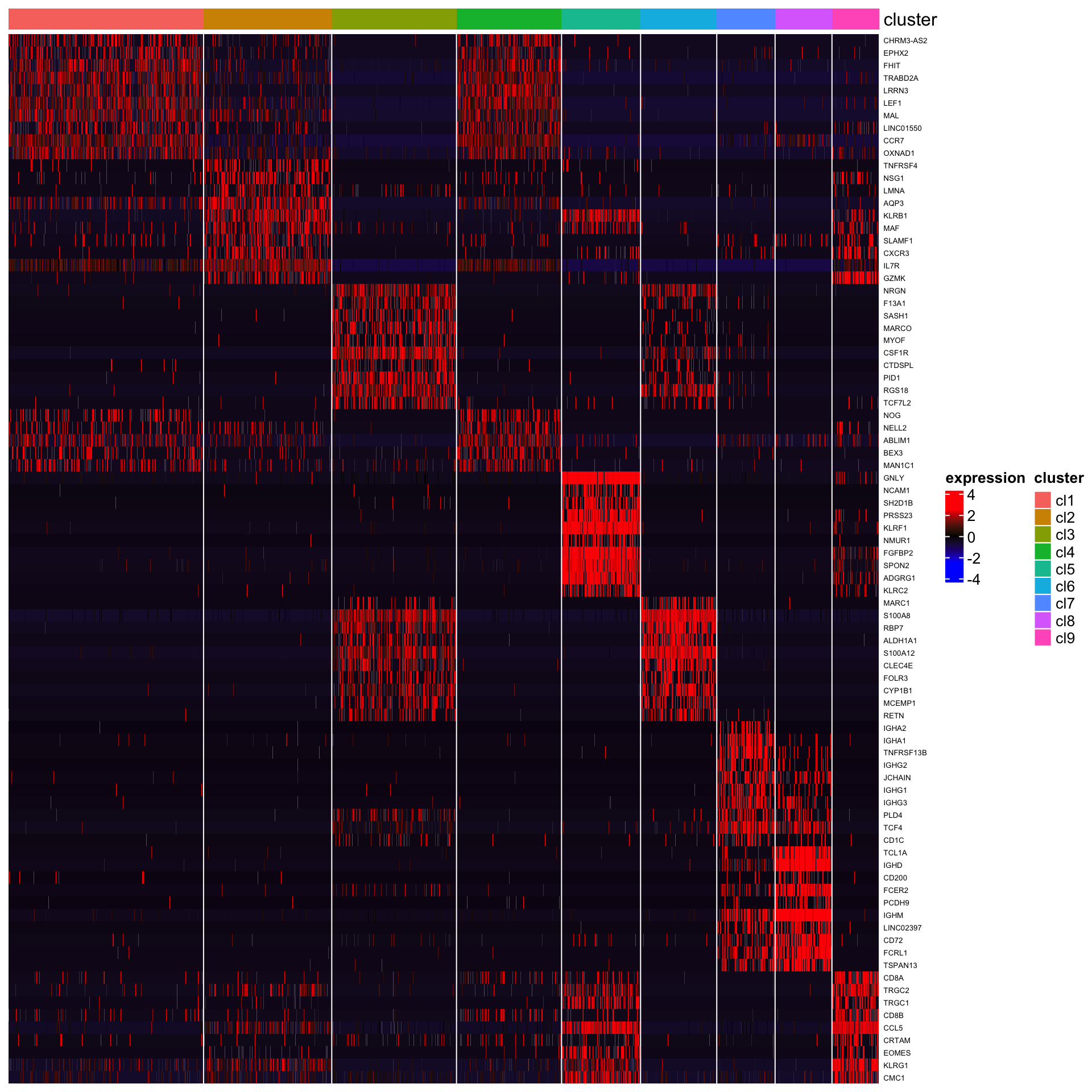
Marker genes can also be extracted as the data frame and can be exported to the text file.
cl3_marker_genes<-getMarkerGenesInfo(PBMCs,cluster.type = "louvain",cluster_id = "cl3")
cl3_marker_genes<-cl3_marker_genes[order(cl3_marker_genes$log2FC,decreasing = T),]
head(cl3_marker_genes)
## Gene ExpA ExpB FoldChange log2FC ExpFreqA ExpFreqB TotalA
## 229 NRGN 7.9109358 0.17166515 46.08353 5.526179 477 289 614
## 153 F13A1 1.1345944 0.05346762 21.22021 4.407367 286 121 614
## 469 SASH1 0.4324292 0.02134311 20.26083 4.340621 230 59 614
## 165 MARCO 0.4954581 0.02503644 19.78948 4.306662 259 73 614
## 316 MYOF 0.3271275 0.01737920 18.82293 4.234419 209 60 614
## 1 CSF1R 2.1105234 0.13134800 16.06818 4.006135 519 254 614
## TotalB ExpFractionA ExpFractionB fishers.pval wilcoxon.pval combined.pval
## 229 3673 0.7768730 0.07868228 9.000920e-295 3.135522e-225 0.000000e+00
## 153 3673 0.4657980 0.03294310 5.466894e-171 2.736062e-269 0.000000e+00
## 469 3673 0.3745928 0.01606316 6.588597e-154 1.254711e-110 5.016038e-261
## 165 3673 0.4218241 0.01987476 5.021125e-172 4.244166e-260 0.000000e+00
## 316 3673 0.3403909 0.01633542 2.480891e-134 3.659939e-182 6.595745e-313
## 1 3673 0.8452769 0.06915328 0.000000e+00 0.000000e+00 0.000000e+00tSNE with identified marker genes
plot_tsne_label_by_genes(PBMCs,gene_list = c("CCR7","CD163","GNLY","CD72"))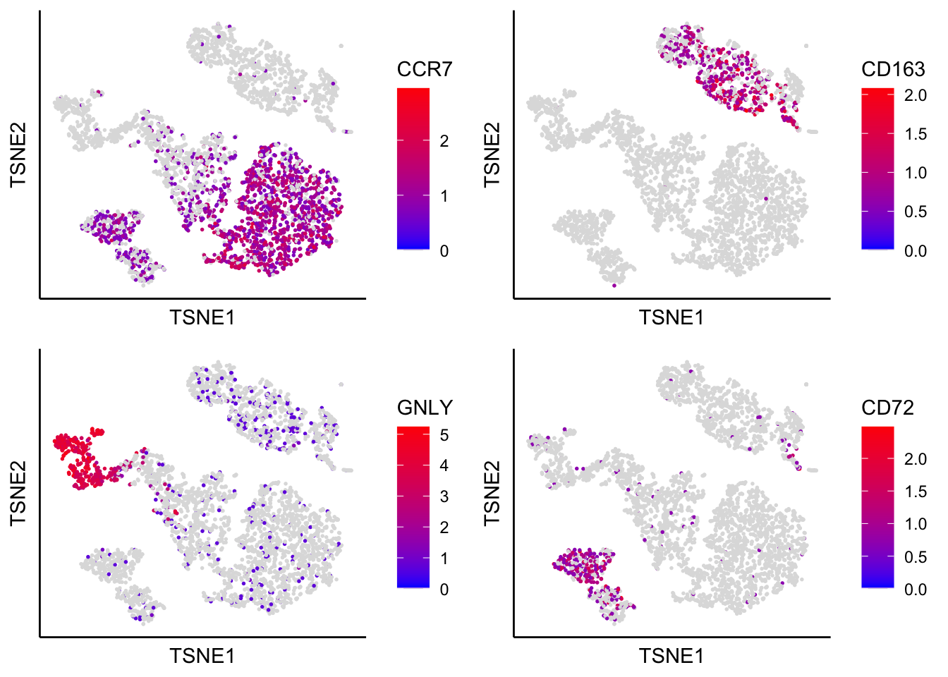
UMAP with identified marker genes
plot_umap_label_by_genes(PBMCs,gene_list = c("CCR7","CD163","GNLY","CD72"))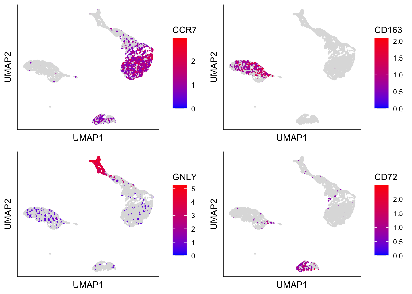
Force-directed graph with identified marker genes
plot_forceDirectedGraph_label_by_genes(PBMCs,gene_list = c("CCR7","CD163","GNLY","CD72"))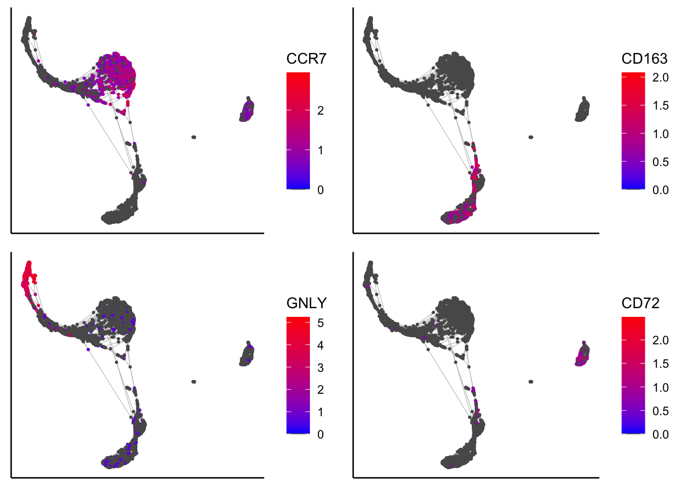
Violin plot for identified marker genes
plot_violin_for_marker_genes(PBMCs,gene_list = c("CCR7","CD163","GNLY","CD72"))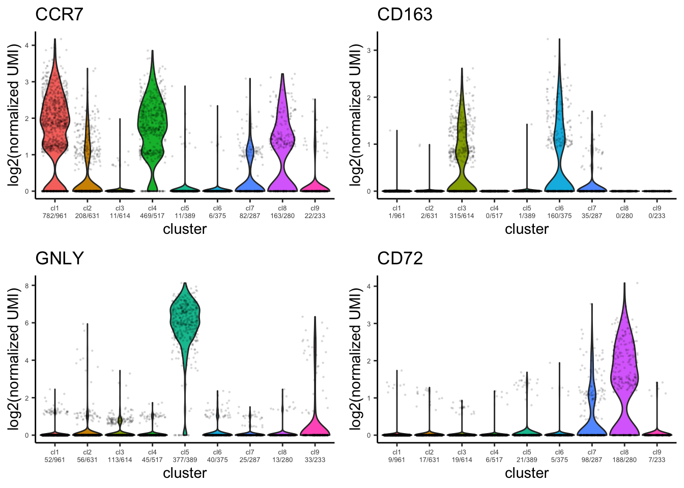
Bubble plot for identified marker genes
plot_bubble_for_genes_per_cluster(PBMCs,cluster.type = "louvain",IsApplyClustering = T,
                            IsClusterByRow = T,IsClusterByColumn = T,
                            gene_list=c("CCR7","CD163",
                                        "GNLY","CD72",
                                        "CD8A","CD8B","IL3RA"
                                        ),show.percent = T,buble.scale = 12,point.color1 = "gray",
                                        point.color2 = "firebrick1")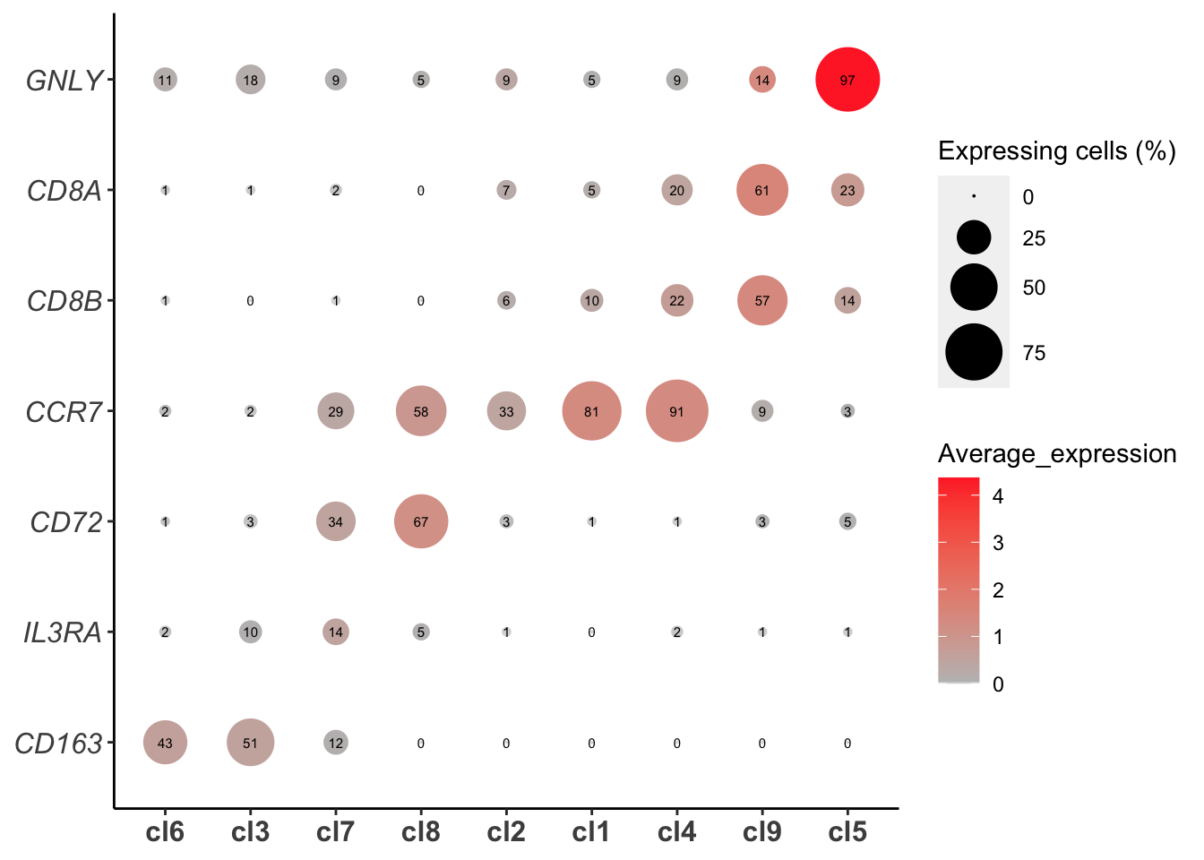
KNN-graph trajectory analysis
SingCellaR also provides an alternative KNN-graph for the trajectory visualization.
runKNN_Graph(PBMCs,n.dims.use = 10,n.neighbors = 10)## [1] "Building Annoy index with metric = euclidean , n_trees = 50"## 0% 10 20 30 40 50 60 70 80 90 100%## [----|----|----|----|----|----|----|----|----|----|## **************************************************|## [1] "Searching Annoy index, search_k = 1000"## 0% 10 20 30 40 50 60 70 80 90 100%
## [----|----|----|----|----|----|----|----|----|----|
## **************************************************|## [1] "Processing graph-layout.."
## [1] "KNN-Graph analysis is done!."KNN-graph visualisation in 3D plot
Plot trajectory in 3D KNN-graph with the clusters
library(threejs)## Loading required package: igraph##
## Attaching package: 'igraph'## The following objects are masked from 'package:stats':
##
## decompose, spectrum## The following object is masked from 'package:base':
##
## unionplot_3D_knn_graph_label_by_clusters(PBMCs,show_method = "louvain",vertext.size = 0.25)Plot trajectory in 3D KNN-graph with a gene of interest
plot_3D_knn_graph_label_by_gene(PBMCs,show.gene = "GNLY",vertext.size = 0.30)K-means clustering based on KNN-graph
K-means clustering can be performed as shown below.
clustering_KMeansOnKNN_Graph(PBMCs, k=10, iter.max = 100)## [1] "KMeans analysis on the KNN-graph is done!."tSNE with K-means clusters
Plot tSNE with identified clusters using K-means clustering.
plot_tsne_label_by_clusters(PBMCs,show_method = "kmeans",point.size = 1)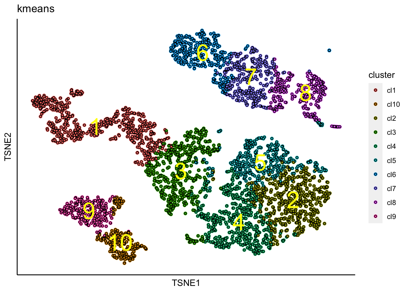
UMAP with identified clusters using K-means clustering.
plot_umap_label_by_clusters(PBMCs,show_method = "kmeans",point.size = 1)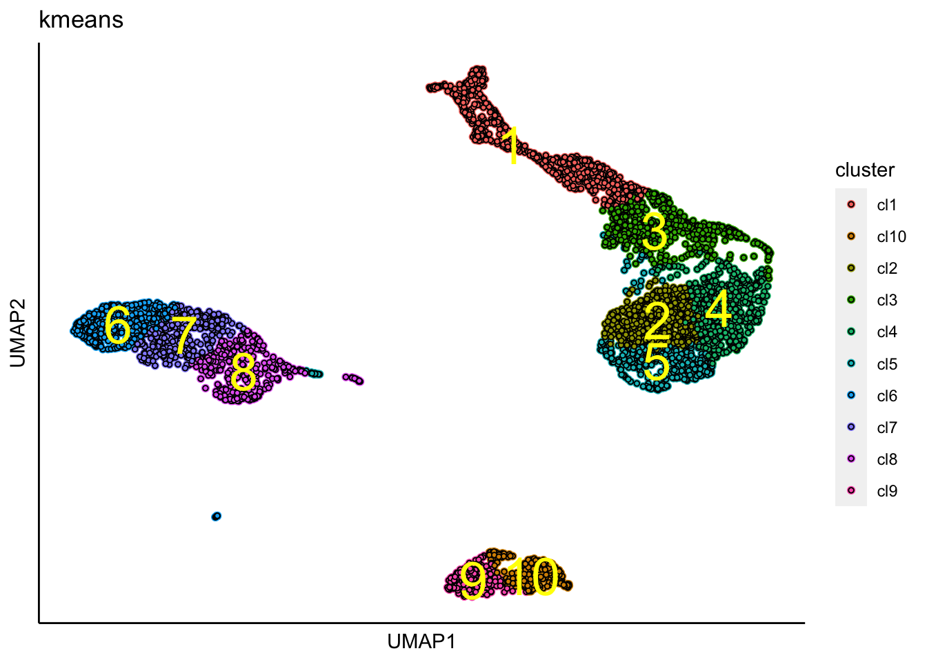
Marker gene identification from K-means clustering
findMarkerGenes(PBMCs,cluster.type = "kmeans")## [1] "Number of genes for analysis: 15911"
## [1] "Creating binary matrix.."
## [1] "Finding differential genes.."
## [1] "Identifying marker genes for: cl1"
## [1] "Processing Fisher's exact test!"
## [1] "Processing Wilcoxon Rank-sum test!"
## [1] "Combining p-values using the fisher's method!"
## [1] "Identifying marker genes for: cl2"
## [1] "Processing Fisher's exact test!"
## [1] "Processing Wilcoxon Rank-sum test!"
## [1] "Combining p-values using the fisher's method!"
## [1] "Identifying marker genes for: cl3"
## [1] "Processing Fisher's exact test!"
## [1] "Processing Wilcoxon Rank-sum test!"
## [1] "Combining p-values using the fisher's method!"
## [1] "Identifying marker genes for: cl4"
## [1] "Processing Fisher's exact test!"
## [1] "Processing Wilcoxon Rank-sum test!"
## [1] "Combining p-values using the fisher's method!"
## [1] "Identifying marker genes for: cl5"
## [1] "Processing Fisher's exact test!"
## [1] "Processing Wilcoxon Rank-sum test!"
## [1] "Combining p-values using the fisher's method!"
## [1] "Identifying marker genes for: cl6"
## [1] "Processing Fisher's exact test!"
## [1] "Processing Wilcoxon Rank-sum test!"
## [1] "Combining p-values using the fisher's method!"
## [1] "Identifying marker genes for: cl7"
## [1] "Processing Fisher's exact test!"
## [1] "Processing Wilcoxon Rank-sum test!"
## [1] "Combining p-values using the fisher's method!"
## [1] "Identifying marker genes for: cl8"
## [1] "Processing Fisher's exact test!"
## [1] "Processing Wilcoxon Rank-sum test!"
## [1] "Combining p-values using the fisher's method!"
## [1] "Identifying marker genes for: cl9"
## [1] "Processing Fisher's exact test!"
## [1] "Processing Wilcoxon Rank-sum test!"
## [1] "Combining p-values using the fisher's method!"
## [1] "Identifying marker genes for: cl10"
## [1] "Processing Fisher's exact test!"
## [1] "Processing Wilcoxon Rank-sum test!"
## [1] "Combining p-values using the fisher's method!"Below is the heatmap of top 10 genes.
plot_heatmap_for_marker_genes(PBMCs,cluster.type = "kmeans",n.TopGenes = 10,rowFont.size = 5)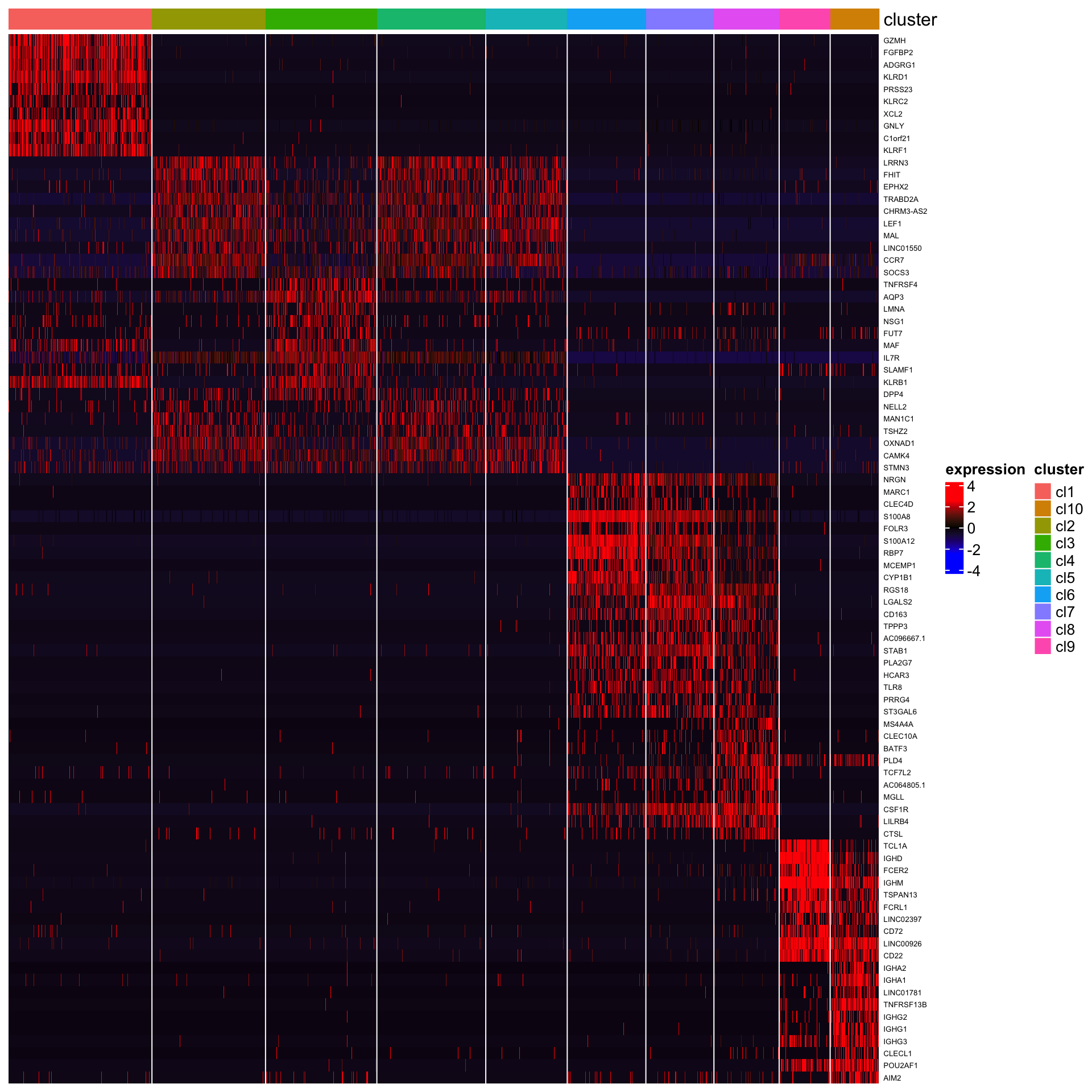
GSEA analysis
GSEA analysis requires pre-ranked genes as the input for gene set enrichment testing. The function below will perform differential gene expression analysis to rank genes based on the combination of log2 of fold change and adjusted p-value.
Preparation for the pre-ranked genes
pre_rankedGenes_for_GSEA<-identifyGSEAPrerankedGenes_for_all_clusters(PBMCs,
                                                                    cluster.type = "louvain")
## [1] "Identifying differentially expressed genes for: cl1"
## [1] "Processing Fisher's exact test!"
## [1] "Identifying differentially expressed genes for: cl2"
## [1] "Processing Fisher's exact test!"
## [1] "Identifying differentially expressed genes for: cl3"
## [1] "Processing Fisher's exact test!"
## [1] "Identifying differentially expressed genes for: cl4"
## [1] "Processing Fisher's exact test!"
## [1] "Identifying differentially expressed genes for: cl5"
## [1] "Processing Fisher's exact test!"
## [1] "Identifying differentially expressed genes for: cl6"
## [1] "Processing Fisher's exact test!"
## [1] "Identifying differentially expressed genes for: cl7"
## [1] "Processing Fisher's exact test!"
## [1] "Identifying differentially expressed genes for: cl8"
## [1] "Processing Fisher's exact test!"
## [1] "Identifying differentially expressed genes for: cl9"
## [1] "Processing Fisher's exact test!"To make this process more efficient, the user might want to save this pre-ranked gene result to the object.
save(pre_rankedGenes_for_GSEA,file="../SingCellaR_example_datasets/10x_genomics_5K_PBMCs/PBMCs_preRankedGenes_for_GSEA.rdata")Run fGSEA
SinceCellaR uses fGSEA (https://bioconductor.org/packages/release/bioc/html/fgsea.html) for the gene set enrichment analysis. This process requires the GMT file that contains gene sets.
Below is an example to perform GSEA using curated gene sets encompass 75 hematopoietic cell types and are available at Zenodo: https://doi.org/10.5281/zenodo.5879071 in GMT file format and are also available in Table S3 from Roy et al., 2021.
load("../SingCellaR_example_datasets/10x_genomics_5K_PBMCs/PBMCs_preRankedGenes_for_GSEA.rdata")
fgsea_Results<-Run_fGSEA_for_multiple_comparisons(GSEAPrerankedGenes_list = pre_rankedGenes_for_GSEA, eps = 0,
                    gmt.file = "../SingCellaR_example_datasets/Human_genesets/human.hematopoiesis.signature.genes.gmt")
## [1] "Processing fGSEA for:cl1"
## [1] "Processing fGSEA for:cl2"
## [1] "Processing fGSEA for:cl3"
## [1] "Processing fGSEA for:cl4"## Warning in fgseaMultilevel(pathways = my.db, stats = prerank.genes, minSize =
## minSize, : There were 1 pathways for which P-values were not calculated properly
## due to unbalanced (positive and negative) gene-level statistic values. For such
## pathways pval, padj, NES, log2err are set to NA. You can try to increase the
## value of the argument nPermSimple (for example set it nPermSimple = 10000)## [1] "Processing fGSEA for:cl5"
## [1] "Processing fGSEA for:cl6"
## [1] "Processing fGSEA for:cl7"
## [1] "Processing fGSEA for:cl8"
## [1] "Processing fGSEA for:cl9"Plot GSEA analysis result
The heatmap below shows only the postive NES score for each gene set compared across clusters.
plot_heatmap_for_fGSEA_all_clusters(fgsea_Results,isApplyCutoff = TRUE,
                                    use_pvalues_for_clustering=T,
                                    show_NES_score = T,fontsize_row = 10,
                                    adjusted_pval = 0.1,
                                    show_only_NES_positive_score = T,format.digits = 3,
                                    clustering_method = "ward.D",
                                    clustering_distance_rows = "euclidean",
                                    clustering_distance_cols = "euclidean",show_text_for_ns = F)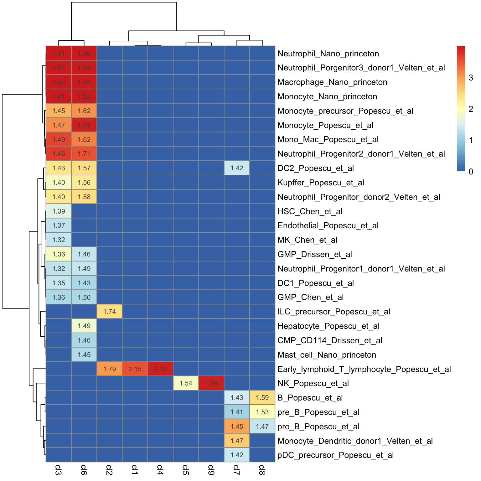
Save SingCellaR object for further analyses
save(PBMCs,file="../SingCellaR_example_datasets/10x_genomics_5K_PBMCs/PBMCs_v0.1.SingCellaR.rdata")