SingCellaR analysis workflow for TARGET-Seq
Loading gene expression table and cell information to SingCellaR object.
First, SingCellaR will be loaded into R, and the ‘SingCellaR’ object is created. The example below shows how to add files from gene expression and cell information into the object.
library(SingCellaR)

MPN<-new("SingCellaR")
MPN@GenesExpressionMatrixFile<-"../SingCellaR_example_datasets/TARGET_Seq/counts_HT_TARGET_GRCh38.v2.txt"
MPN@CellsMetaDataFile<-"../SingCellaR_example_datasets/TARGET_Seq/HT_TARGETseq_colData.qc_Ghr38.txt"
load_gene_expression_from_a_file(MPN,isTargetSeq = T,sep="\t")
## [1] "The sparse matrix is created."MPN## An object of class SingCellaR with a matrix of : 33514 genes across 3593 samples.Next, cell information will be processed. The percentage of mitochondrial per cell will be calculated. For human, mitochondrial gene names start with “MT-”.
The ERCC genes must be specify with the parameter ‘ERCC_genes_start_with’, if ERCC spike-in is incorporated.
TargetSeq_process_cells_annotation(MPN,mito_genes_start_with  = "MT-",
                                   ERCC_genes_start_with = "ERCC-")
## [1] "List of mitochondrial genes:"
## [1] "MT-ND1" "MT-ND2" "MT-CO1" "MT-CO2" "MT-ATP8" "MT-ATP6" "MT-CO3"
## [8] "MT-ND3" "MT-ND4L" "MT-ND4" "MT-ND5" "MT-ND6" "MT-CYB"
## [1] "List of ERCC:"
## character(0)
## [1] "The meta data is processed."QC plots for TARGET-Seq data
TargetSeq_plot_cells_annotation(MPN,type = "boxplot")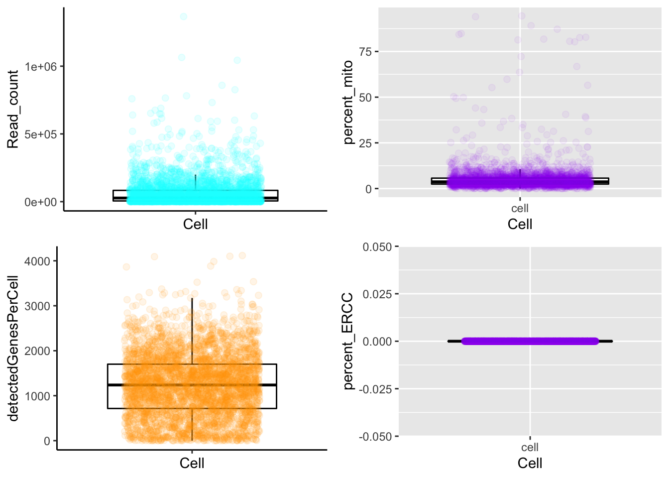
Filtering
TargetSeq_filter_cells_and_genes(MPN,min_Reads = 2000,
                                 max_percent_mito = 10,
                                 genes_with_expressing_cells = 10,max_percent_ERCC = 50)
## [1] "The cells and genes metadata are updated by adding the filtering status."
## [1] "835/3593 cells will be filtered out from the downstream analyses!."Loading external cell metadata (e.g., genotyping data)
To load the cell metadata information from TARGET-Seq cell information, the following function will be performed.
TargetSeq_load_cell_metadata(MPN,sep = "\t",a_column_of_the_cell_names = 1)## [1] "The cell metadata is updated!"Checking the updated metadata.
head(MPN@meta.data)## Cell sampleID UMI_count detectedGenesPerCell percent_mito percent_ERCC
## 1 TR4PL21_11B 2595 834 2.466281 0
## 2 TR4PL21_11C 4859 632 5.412636 0
## 3 TR4PL21_11D 5300 670 2.264151 0
## 4 TR4PL21_11E 5251 1271 3.599314 0
## 5 TR4PL21_11F 2282 798 3.637160 0
## 6 TR4PL21_11L 20403 1801 4.170955 0
## IsPassed cell.type donor timepoint donor.type primer.mix batch plate
## 1 TRUE cd34+ IF0137 baseline patient IF0137_mix batch_1 TR4PL21
## 2 TRUE cd34+ IF0137 baseline patient IF0137_mix batch_1 TR4PL21
## 3 TRUE cd34+ IF0137 baseline patient IF0137_mix batch_1 TR4PL21
## 4 TRUE cd34+ IF0137 baseline patient IF0137_mix batch_1 TR4PL21
## 5 TRUE cd34+ IF0137 baseline patient IF0137_mix batch_1 TR4PL21
## 6 TRUE cd34+ IF0137 baseline patient IF0137_mix batch_1 TR4PL21
## pool CD45RA CD90 CD38 lineage.viability CD34 CD123
## 1 TR4PL21_Q2 1502.17 2621.87 5156.63 12043.33 29906.12 3428.90
## 2 TR4PL21_Q1 1782.70 1887.77 14743.83 16879.47 21457.04 1700.39
## 3 TR4PL21_Q2 995.36 1545.84 7552.66 4882.79 17353.63 1342.27
## 4 TR4PL21_Q1 748.31 16677.71 11011.12 14496.51 29338.79 3951.90
## 5 TR4PL21_Q2 1348.57 2874.07 19794.60 12866.39 18098.87 2719.89
## 6 TR4PL21_Q2 2213.63 2963.91 37265.15 18894.65 10691.38 649.52
## genotypesall qcgenotype genes.detected
## 1 JAK2_HET_U2AF1_HET_TET2_pI1105_HET_ASXL1_p910_HET TRUE 839
## 2 JAK2_HET_U2AF1_HET_ASXL1_p910_HET TRUE 636
## 3 JAK2_HET_U2AF1_HET TRUE 702
## 4 JAK2_HET_U2AF1_HET_ASXL1_p897_HET TRUE 1250
## 5 JAK2_HET_U2AF1_HET_TET2_pI1105_HET_ASXL1_p910_HET TRUE 812
## 6 JAK2_HOM_U2AF1_HET TRUE 1830
## input.reads unique.mapped multimap MReads lib.size unmapped ercc.count
## 1 7566 4235 551 131 2741 2780 134
## 2 17580 10089 1658 445 5561 5833 696
## 3 16977 10024 1497 296 6301 5456 554
## 4 39883 9074 1282 336 5614 29527 354
## 5 30008 4791 658 158 2450 24559 177
## 6 46909 29782 4315 1330 21983 12812 748
## pc.uniquemapped pc.multimap pc.unmapped pc.ingenes pc.ercc pc.mit.reads
## 1 0.5597409 0.07282580 0.3674333 0.6472255 0.04888727 0.017314301
## 2 0.5738908 0.09431172 0.3317975 0.5511944 0.12515735 0.025312856
## 3 0.5904459 0.08817812 0.3213760 0.6285914 0.08792255 0.017435354
## 4 0.2275155 0.03214402 0.7403405 0.6186908 0.06305664 0.008424642
## 5 0.1596574 0.02192749 0.8184151 0.5113755 0.07224490 0.005265263
## 6 0.6348888 0.09198661 0.2731246 0.7381304 0.03402629 0.028352768
## genotype.class rnaseq.qc qc.all
## 1 realclone TRUE TRUE
## 2 realclone TRUE TRUE
## 3 realclone TRUE TRUE
## 4 realclone TRUE TRUE
## 5 realclone TRUE TRUE
## 6 realclone TRUE TRUEMore filtering based on updated cells information
The TARGET-Seq analysis (developed by Rodriguez-Meira et al., Mol. Cell, 2019) provides QC information of cells. Therefore, those cells information will be included for further filtering.
- Library size > 2000 reads
- The percentage of mitochondrial reads < 10%
- The percentage of ERCC reads < 50%
- The number of detected genes per cell > 500
my.cell_info<-subset(MPN@meta.data,qc.all=="TRUE")
my.cell_filtered<-subset(my.cell_info, UMI_count > 2000 & percent_mito < 10 & detectedGenesPerCell > 500 & pc.ercc < 50)
nrow(my.cell_filtered)
## [1] 2679It is critical to add “IsPassed==TRUE” to the cells that pass QC.
my.cell_info$IsPassed[my.cell_info$Cell %in% my.cell_filtered$Cell]<-TRUE
table(my.cell_info$IsPassed)
##
## FALSE TRUE
## 119 2679Finally, the slot ‘meta.data’ in the MPN object will be updated.
MPN@meta.data<-my.cell_infoClassification of cells base on genotypes
Next, to reproduce Figure 5a found in Rodriguez-Meira et al., Mol. Cell, 2019, the mutation information is separated into distinct genotyping categories as shown below.
cell_metadata<-get_cells_annotation(MPN)
cell_metadata$genotype_class1<-"NA"

JAK2_only<-c("\\bJAK2_HET\\b","\\bJAK2_HOM\\b")
cell_metadata$genotype_class1[grep(paste(JAK2_only,collapse="|"),cell_metadata$genotypesall)]<-"JAK2_only"

WT_normal<-c("\\bWT\\b")
cell_metadata$genotype_class1[grep(paste(WT_normal,collapse="|"),cell_metadata$genotypesall)]<-"WT_normal"

WT_patient<-c("\\bJAK2_WT\\b")
cell_metadata$genotype_class1[grep(paste(WT_patient,collapse="|"),cell_metadata$genotypesall)]<-"WT_patient"

JAK2_spliceosome<-c("JAK2_HET_SRSF2_HET","JAK2_HET_U2AF1_HET","JAK2_HOM_CBL_p404_HET_SRSF2_HET","JAK2_HOM_SF3B1_HET","JAK2_HOM_SRSF2_HET",
                    "JAK2_HOM_U2AF1_HET")
cell_metadata$genotype_class1[grep(paste(JAK2_spliceosome,collapse="|"),cell_metadata$genotypesall)]<-"JAK2_spliceosome"

JAK2_spliceosome_epigenetic<-c("JAK2_HET_U2AF1_HET_ASXL1_p910_HET","JAK2_HET_U2AF1_HET_TET2_pI1105_HET_ASXL1_p910_HET",
                               "JAK2_HET_U2AF1_HET_ASXL1_p897_HET")
cell_metadata$genotype_class1[grep(paste(JAK2_spliceosome_epigenetic,collapse="|"),cell_metadata$genotypesall)]<-"JAK2_spliceosome_epigenetic"

JAK2_epigenetic<-c("JAK2_HOM_ASXL1_p644_HET","JAK2_HOM_TET2_p1612_HET")
cell_metadata$genotype_class1[grep(paste(JAK2_epigenetic,collapse="|"),cell_metadata$genotypesall)]<-"JAK2_epigenetic"

cell_metadata_for_analysis<-subset(cell_metadata,genotype_class1!="NA") #2742 cells considered for this analysis

nrow(cell_metadata_for_analysis)
## [1] 2742Update cell information
MPN@meta.data<-cell_metadata_for_analysisData normalization
To normalize TARGET-Seq data, the parameter ‘use.scaled.factor’ has to be set up as ‘FALSE’. This is to normalize by the average of library sizes.
normalize_UMIs(MPN,use.scaled.factor = F)## [1] "Normalization is completed!."Identify variable genes
get_variable_genes_by_fitting_GLM_model(MPN,mean_expr_cutoff = 1,disp_zscore_cutoff = 0.05,
                                        quantile_genes_expr_for_fitting = 0.5,
                                        quantile_genes_cv2_for_fitting =0.3)
## [1] "Calculate row variance.."
##
|
| | 0%
|
|========= | 12%
|
|================== | 25%
|
|========================== | 38%
|
|=================================== | 50%
|
|============================================ | 62%
|
|==================================================== | 75%
|
|============================================================= | 88%
|
|======================================================================| 100%[1] "Using :4696 genes for fitting the GLM model!"
## [1] "Identified :3639 variable genes"remove_unwanted_genes_from_variable_gene_set(MPN,gmt.file = "../SingCellaR_example_datasets/Human_genesets/human.ribosomal-mitocondrial.genes.gmt",
removed_gene_sets=c("Ribosomal_gene","Mitocondrial_gene"))## [1] "6 genes are removed from the variable gene set."Here, the plot shows highly variable genes (cyan) in the fitted GLM model.
plot_variable_genes(MPN,quantile_genes_expr_for_fitting = 0.5,quantile_genes_cv2_for_fitting =0.3)## [1] "Calculate row variance.."
##
|
| | 0%
|
|========= | 12%
|
|================== | 25%
|
|========================== | 38%
|
|=================================== | 50%
|
|============================================ | 62%
|
|==================================================== | 75%
|
|============================================================= | 88%
|
|======================================================================| 100%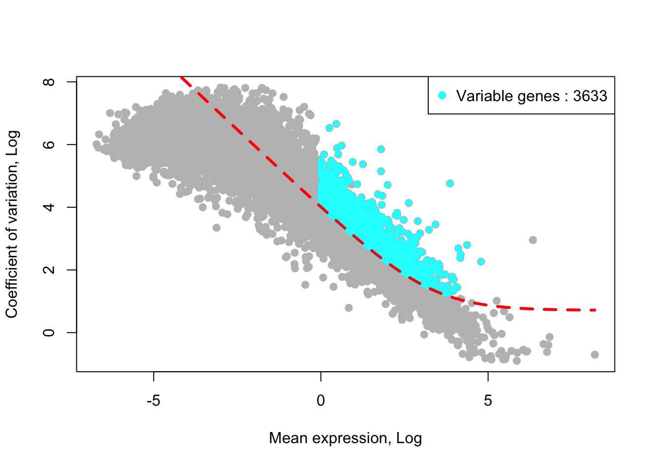 ## PCA anlysis
runPCA(MPN,use.components=30,use.regressout.data = F)## [1] "PCA analysis is done!."Next, the number of PCs used for downstream analyses will be determined from the scree plot.
plot_PCA_Elbowplot(MPN)
UMAP analysis
runUMAP(MPN,dim_reduction_method = "pca",n.dims.use = 10,n.neighbors = 20,
        uwot.metric = "euclidean")
## 17:37:33 UMAP embedding parameters a = 1.121 b = 1.057## 17:37:33 Read 2626 rows and found 10 numeric columns## 17:37:33 Using Annoy for neighbor search, n_neighbors = 20## 17:37:33 Building Annoy index with metric = euclidean, n_trees = 50## 0% 10 20 30 40 50 60 70 80 90 100%## [----|----|----|----|----|----|----|----|----|----|## **************************************************|
## 17:37:33 Writing NN index file to temp file /var/folders/c6/_w309xr54n7cphf9nw4x_ms40000gn/T//Rtmp0EVVqP/filecde23596aaf1
## 17:37:33 Searching Annoy index using 8 threads, search_k = 2000
## 17:37:34 Annoy recall = 100%
## 17:37:34 Commencing smooth kNN distance calibration using 8 threads with target n_neighbors = 20
## 17:37:35 Initializing from normalized Laplacian + noise (using irlba)
## 17:37:35 Commencing optimization for 500 epochs, with 67982 positive edges
## 17:37:38 Optimization finished## [1] "UMAP analysis is done!."plot_umap_label_by_a_feature_of_interest(MPN,feature = "donor",point.size = 1)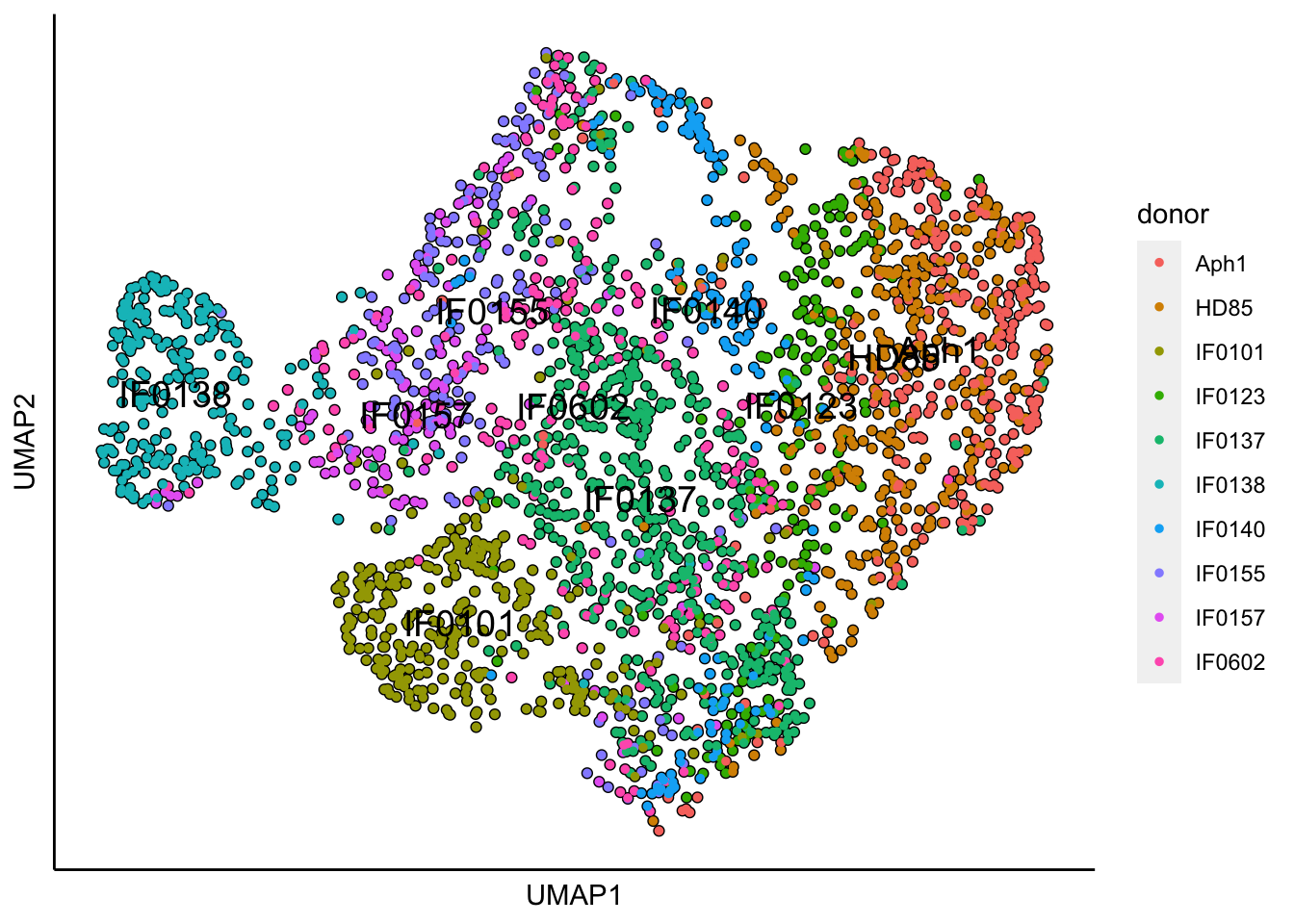
plot_umap_label_by_a_feature_of_interest(MPN,feature = "donor.type",point.size = 1)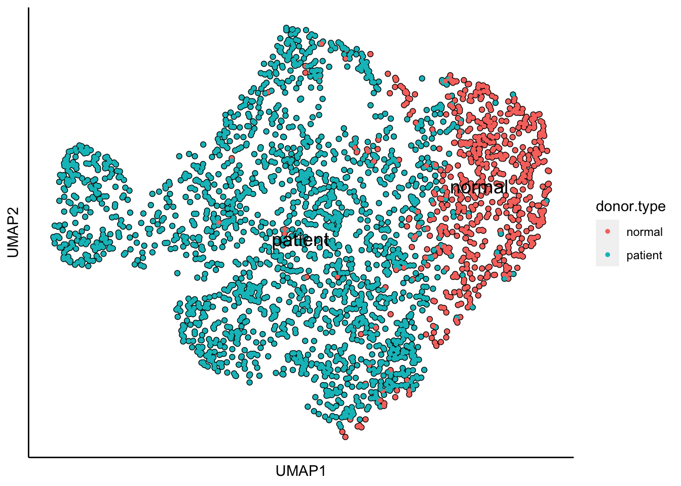
plot_umap_label_by_a_feature_of_interest(MPN,feature = "batch",point.size = 1)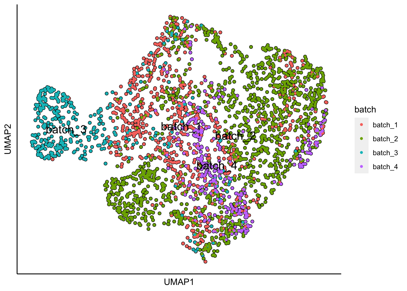
plot_umap_label_by_a_feature_of_interest(MPN,feature = "genotype_class1",point.size = 1)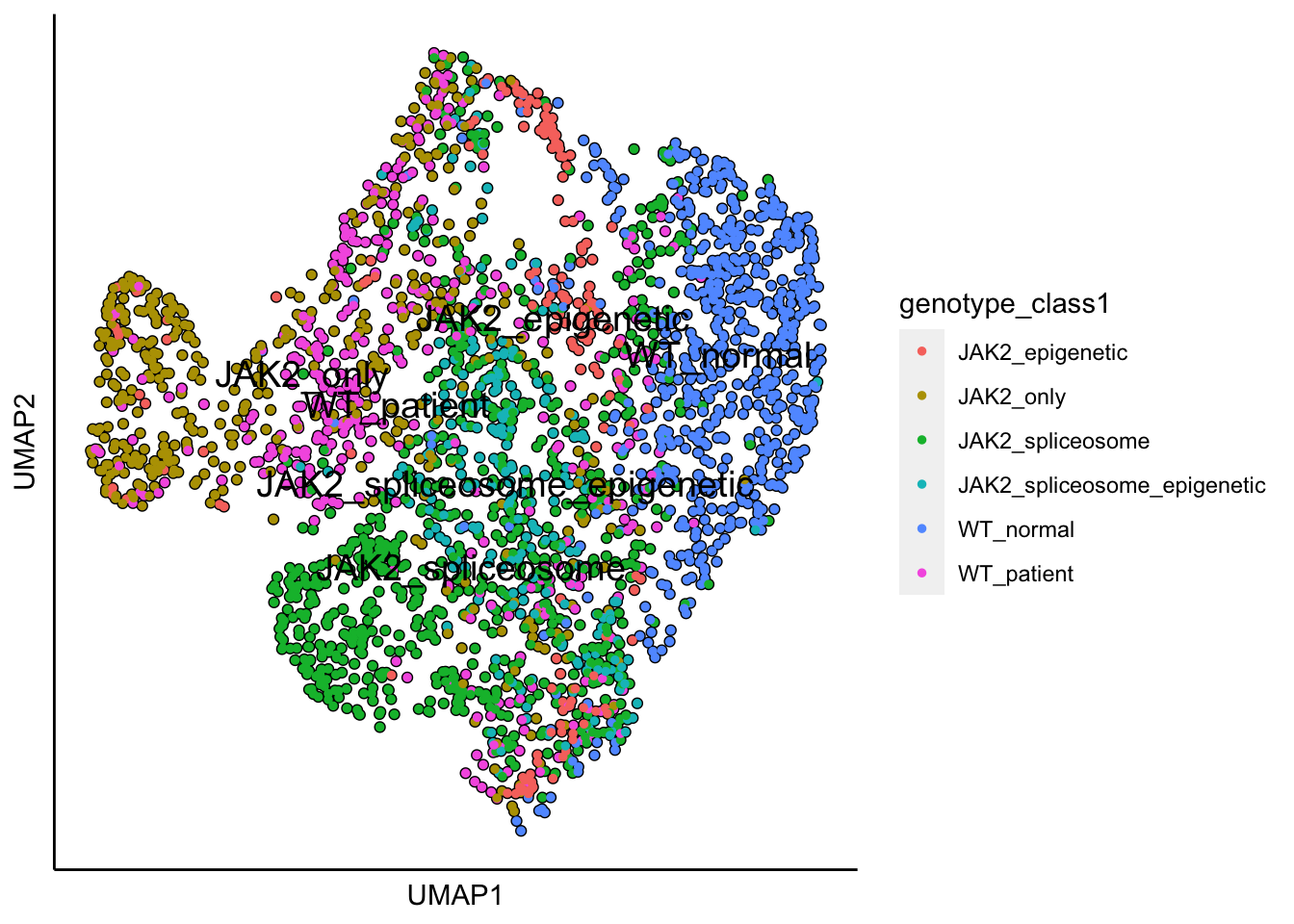
Regressing out the source of variations and preserving genotypes of interest
UMAP plots show batch and donor effects. Limma will be used to preserve the genotypes of interest and to regress out batch and donor effects.
remove_unwanted_confounders(MPN,residualModelFormulaStr = "~donor+batch",
                            preserved_feature = "~genotype_class1")
##
|
| | 0%Coefficients not estimable: (Intercept) donorIF0602## Warning: Partial NA coefficients for 2000 probe(s)##
|
|==== | 6%Coefficients not estimable: (Intercept) donorIF0602## Warning: Partial NA coefficients for 2000 probe(s)##
|
|======== | 12%Coefficients not estimable: (Intercept) donorIF0602## Warning: Partial NA coefficients for 2000 probe(s)##
|
|============ | 18%Coefficients not estimable: (Intercept) donorIF0602## Warning: Partial NA coefficients for 2000 probe(s)##
|
|================ | 24%Coefficients not estimable: (Intercept) donorIF0602## Warning: Partial NA coefficients for 2000 probe(s)##
|
|===================== | 29%Coefficients not estimable: (Intercept) donorIF0602## Warning: Partial NA coefficients for 2000 probe(s)##
|
|========================= | 35%Coefficients not estimable: (Intercept) donorIF0602## Warning: Partial NA coefficients for 2000 probe(s)##
|
|============================= | 41%Coefficients not estimable: (Intercept) donorIF0602## Warning: Partial NA coefficients for 2000 probe(s)##
|
|================================= | 47%Coefficients not estimable: (Intercept) donorIF0602## Warning: Partial NA coefficients for 2000 probe(s)##
|
|===================================== | 53%Coefficients not estimable: (Intercept) donorIF0602## Warning: Partial NA coefficients for 2000 probe(s)##
|
|========================================= | 59%Coefficients not estimable: (Intercept) donorIF0602## Warning: Partial NA coefficients for 2000 probe(s)##
|
|============================================= | 65%Coefficients not estimable: (Intercept) donorIF0602## Warning: Partial NA coefficients for 2000 probe(s)##
|
|================================================= | 71%Coefficients not estimable: (Intercept) donorIF0602## Warning: Partial NA coefficients for 2000 probe(s)##
|
|====================================================== | 76%Coefficients not estimable: (Intercept) donorIF0602## Warning: Partial NA coefficients for 2000 probe(s)##
|
|========================================================== | 82%Coefficients not estimable: (Intercept) donorIF0602## Warning: Partial NA coefficients for 2000 probe(s)##
|
|============================================================== | 88%Coefficients not estimable: (Intercept) donorIF0602## Warning: Partial NA coefficients for 2000 probe(s)##
|
|================================================================== | 94%Coefficients not estimable: (Intercept) donorIF0602## Warning: Partial NA coefficients for 1514 probe(s)##
|
|======================================================================| 100%
## [1] "Removing unwanted sources of variation is done!"PCA anlysis after regressing out donor and batch effects
runPCA(MPN,use.components=30,use.regressout.data = T)## [1] "PCA analysis is done!."Next, the number of PCs used for downstream analyses will be determined from the scree plot.
plot_PCA_Elbowplot(MPN)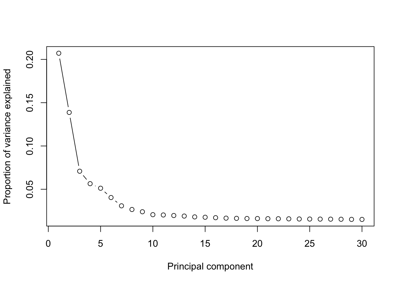
UMAP analysis after regressing out batche and donor effects
runUMAP(MPN,dim_reduction_method = "pca",n.dims.use = 10,n.neighbors = 20,
        uwot.metric = "euclidean")
## 17:38:08 UMAP embedding parameters a = 1.121 b = 1.057## 17:38:08 Read 2626 rows and found 10 numeric columns## 17:38:08 Using Annoy for neighbor search, n_neighbors = 20## 17:38:08 Building Annoy index with metric = euclidean, n_trees = 50## 0% 10 20 30 40 50 60 70 80 90 100%## [----|----|----|----|----|----|----|----|----|----|## **************************************************|
## 17:38:08 Writing NN index file to temp file /var/folders/c6/_w309xr54n7cphf9nw4x_ms40000gn/T//Rtmp0EVVqP/filecde2cfb06bf
## 17:38:08 Searching Annoy index using 8 threads, search_k = 2000
## 17:38:08 Annoy recall = 100%
## 17:38:09 Commencing smooth kNN distance calibration using 8 threads with target n_neighbors = 20
## 17:38:10 Initializing from normalized Laplacian + noise (using irlba)
## 17:38:10 Commencing optimization for 500 epochs, with 70486 positive edges
## 17:38:13 Optimization finished## [1] "UMAP analysis is done!."plot_umap_label_by_a_feature_of_interest(MPN,feature = "donor",point.size = 1)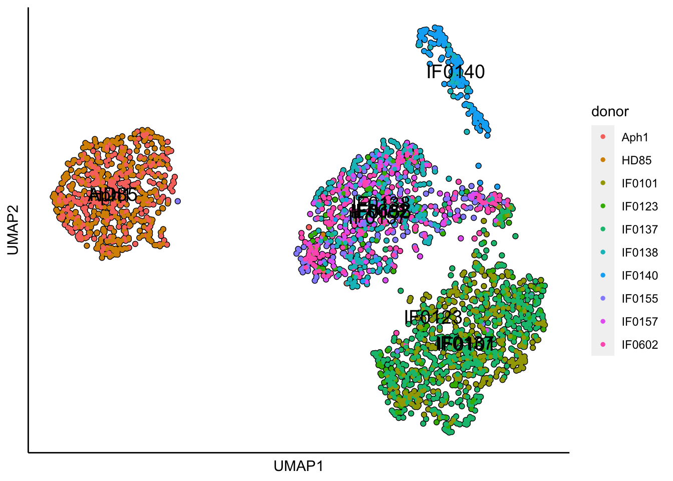
plot_umap_label_by_a_feature_of_interest(MPN,feature = "donor.type",point.size = 1)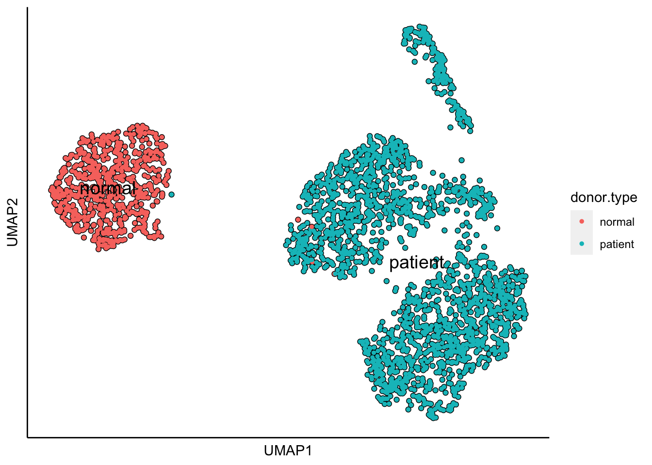
plot_umap_label_by_a_feature_of_interest(MPN,feature = "batch",point.size = 1)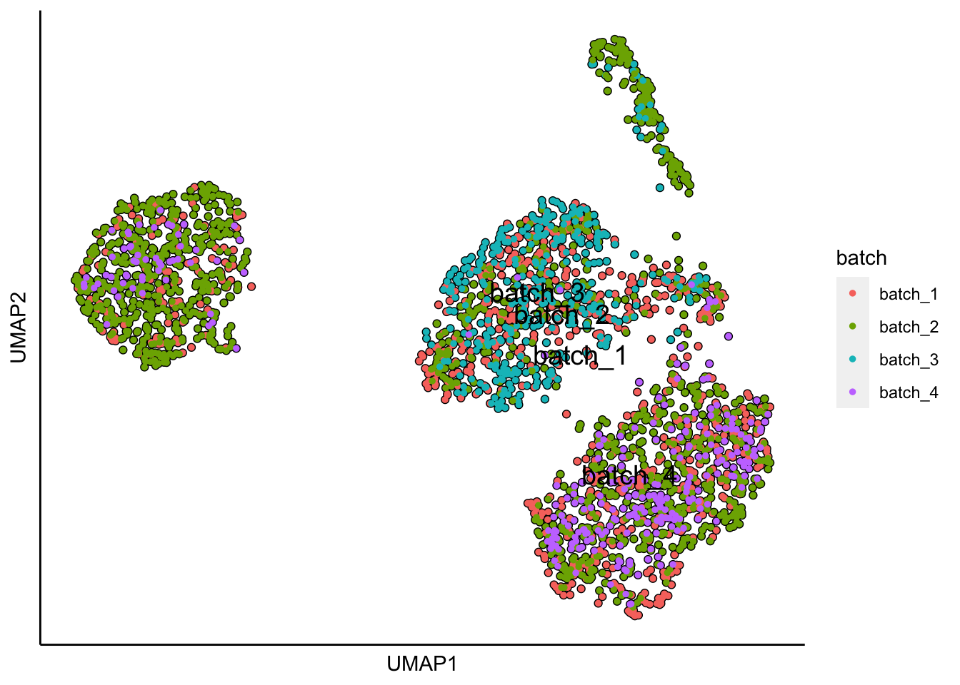
plot_umap_label_by_a_feature_of_interest(MPN,feature = "genotype_class1",point.size = 1)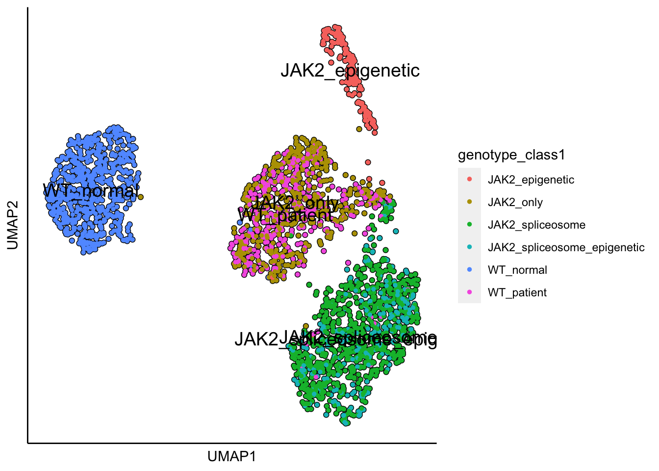
tSNE analysis after regressing out batche and donor effects
runTSNE(MPN,dim_reduction_method = "pca",n.dims.use = 10)## [1] "TSNE analysis is done!."plot_tsne_label_by_a_feature_of_interest(MPN,feature = "genotype_class1",point.size = 1)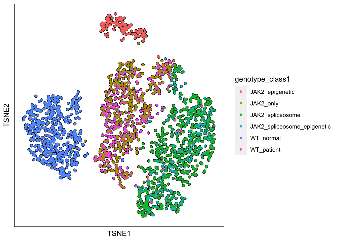
Force-directed graph analysis
runFA2_ForceDirectedGraph(MPN,dim_reduction_method = "pca",n.dims.use = 10)## [1] "Building Annoy index with metric = euclidean , n_trees = 50"## 0% 10 20 30 40 50 60 70 80 90 100%## [----|----|----|----|----|----|----|----|----|----|## **************************************************|## [1] "Searching Annoy index, search_k = 500"## 0% 10 20 30 40 50 60 70 80 90 100%
## [----|----|----|----|----|----|----|----|----|----|
## **************************************************|## [1] "Processing fa2.."
## [1] "Force directed graph analysis is done!."plot_forceDirectedGraph_label_by_a_feature_of_interest(MPN,feature = "genotype_class1",
background.color = "black",vertex.size = 1)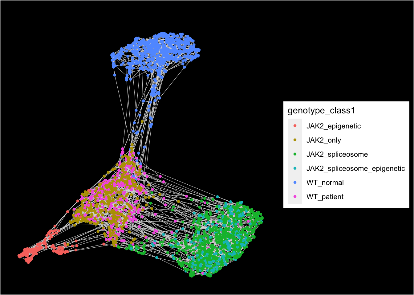
Differential gene expression analysis
Below is an example of how to perform differential gene expression analysis between ‘WT_normal’ and ‘WT_patient’.
First, cell names per each group will be extracted from the cell metadata.
WT_normal.cells<-subset(MPN@meta.data,genotype_class1=="WT_normal")
WT_normal.cell_ids<-WT_normal.cells$Cell

WT_patient.cells<-subset(MPN@meta.data,genotype_class1=="WT_patient")
WT_patient.cell_ids<-WT_patient.cells$Cell
Second, differential gene expression analysis will be performed.
DE.genes<-identifyDifferentialGenes(objectA = MPN, objectB = MPN, cellsA = WT_normal.cell_ids, cellsB = WT_patient.cell_ids)## [1] "Processing Fisher's exact test!"
## [1] "Processing Wilcoxon Rank-sum test!"
## [1] "Combining p-values using the fisher's method!"head(DE.genes)## Gene ExpA ExpB FoldChange log2FC ExpFreqA
## GIMAP7 GIMAP7 38.6958440 0.5000682 77.38113053 6.273910 339
## AC123912.4 AC123912.4 0.3018886 4.8313286 0.06248562 -4.000332 39
## DYNLL1 DYNLL1 35.6631112 5.1568363 6.91569576 2.789874 430
## CNOT1 CNOT1 1.5126984 4.3828158 0.34514304 -1.534734 122
## ELMSAN1 ELMSAN1 8.3102311 66.4716260 0.12501922 -2.999778 228
## BTG3 BTG3 1.6659861 17.8049370 0.09356877 -3.417829 67
## ExpFreqB TotalA TotalB ExpFractionA ExpFractionB fishers.pval
## GIMAP7 8 678 388 0.50000000 0.02061856 1.805764e-72
## AC123912.4 165 678 388 0.05752212 0.42525773 4.721279e-48
## DYNLL1 72 678 388 0.63421829 0.18556701 1.479443e-47
## CNOT1 223 678 388 0.17994100 0.57474227 1.669020e-39
## ELMSAN1 276 678 388 0.33628319 0.71134021 1.174696e-32
## BTG3 158 678 388 0.09882006 0.40721649 1.614010e-31
## wilcoxon.pval combined.pval adjusted.pval
## GIMAP7 1.510069e-56 8.036717e-126 7.321449e-123
## AC123912.4 3.775491e-50 3.988782e-95 1.816890e-92
## DYNLL1 3.099438e-49 1.011206e-93 3.070695e-91
## CNOT1 2.950290e-38 8.701114e-75 1.981679e-72
## ELMSAN1 1.841131e-38 3.490915e-68 6.360447e-66
## BTG3 3.340895e-35 8.157683e-64 1.238608e-61Filtering DE genes
sig.genes<-subset(DE.genes,adjusted.pval < 0.05 & (ExpFractionA > 0.25 | ExpFractionB > 0.25) & abs(log2FC) > 2)
sig.genes<-sig.genes[order(abs(sig.genes$log2FC),decreasing = T),]
sig.genes
## Gene ExpA ExpB FoldChange log2FC ExpFreqA
## GIMAP7 GIMAP7 38.6958440 0.5000682 77.38113053 6.273910 339
## CRIP2 CRIP2 31.1294075 1.7242098 18.05430325 4.174271 223
## AC123912.4 AC123912.4 0.3018886 4.8313286 0.06248562 -4.000332 39
## BTG3 BTG3 1.6659861 17.8049370 0.09356877 -3.417829 67
## SKIL SKIL 0.7104263 7.0709176 0.10047159 -3.315140 40
## SLF2 SLF2 10.8691048 1.2081164 8.99673633 3.169402 219
## PIM1 PIM1 7.5085602 0.9114636 8.23791578 3.042279 237
## ELMSAN1 ELMSAN1 8.3102311 66.4716260 0.12501922 -2.999778 228
## EGR1 EGR1 1.3225500 9.8840059 0.13380708 -2.901774 84
## MGAT4A MGAT4A 2.3922515 17.2830979 0.13841566 -2.852921 66
## MXD1 MXD1 1.1978888 8.6463778 0.13854227 -2.851602 56
## PCIF1 PCIF1 2.3637255 16.3510228 0.14456133 -2.790246 138
## DYNLL1 DYNLL1 35.6631112 5.1568363 6.91569576 2.789874 430
## S100A11 S100A11 3.9074935 0.5964116 6.55167268 2.711863 209
## HMGA2 HMGA2 2.7493416 17.9785942 0.15292306 -2.709122 95
## ID2 ID2 6.4516358 41.4028446 0.15582591 -2.681993 159
## RALA RALA 14.8178047 2.4676061 6.00493123 2.586148 262
## DDIT3 DDIT3 3.1722772 18.9953501 0.16700283 -2.582056 100
## SBDS SBDS 3.3994358 17.6993364 0.19206572 -2.380328 137
## UCP2 UCP2 45.5663838 8.8673749 5.13865538 2.361391 454
## IRF1 IRF1 4.5471141 22.9399835 0.19821784 -2.334841 221
## UNK UNK 3.0216109 15.0597733 0.20064120 -2.317310 72
## BZW1 BZW1 1.6276372 7.7135384 0.21101045 -2.244614 151
## AC243960.1 AC243960.1 10.2966047 2.1899288 4.70179892 2.233213 215
## RIPK2 RIPK2 2.7190740 12.4159585 0.21899832 -2.191008 116
## MTRNR2L1 MTRNR2L1 0.7515776 3.4255535 0.21940325 -2.188343 234
## TSPAN2 TSPAN2 9.0709179 2.0270495 4.47493646 2.161867 233
## S100A10 S100A10 32.1952894 7.5423327 4.26861166 2.093767 289
## EIF1B EIF1B 8.0837818 34.1970180 0.23638850 -2.080768 183
## LMNA LMNA 16.3573412 3.8988413 4.19543653 2.068821 266
## KLF10 KLF10 2.6063906 10.7717852 0.24196459 -2.047132 105
## ATP2C1 ATP2C1 4.2478195 17.3833964 0.24436074 -2.032916 175
## CCDC59 CCDC59 2.5513051 10.4129832 0.24501193 -2.029076 93
## PBXIP1 PBXIP1 17.3560146 4.2832509 4.05206585 2.018658 351
## ExpFreqB TotalA TotalB ExpFractionA ExpFractionB fishers.pval
## GIMAP7 8 678 388 0.50000000 0.02061856 1.805764e-72
## CRIP2 23 678 388 0.32890855 0.05927835 3.139866e-27
## AC123912.4 165 678 388 0.05752212 0.42525773 4.721279e-48
## BTG3 158 678 388 0.09882006 0.40721649 1.614010e-31
## SKIL 127 678 388 0.05899705 0.32731959 6.545259e-30
## SLF2 30 678 388 0.32300885 0.07731959 3.767417e-22
## PIM1 34 678 388 0.34955752 0.08762887 2.870212e-23
## ELMSAN1 276 678 388 0.33628319 0.71134021 1.174696e-32
## EGR1 127 678 388 0.12389381 0.32731959 5.568782e-15
## MGAT4A 125 678 388 0.09734513 0.32216495 2.923309e-19
## MXD1 122 678 388 0.08259587 0.31443299 1.244670e-21
## PCIF1 177 678 388 0.20353982 0.45618557 1.240317e-17
## DYNLL1 72 678 388 0.63421829 0.18556701 1.479443e-47
## S100A11 23 678 388 0.30825959 0.05927835 3.116649e-24
## HMGA2 140 678 388 0.14011799 0.36082474 2.421682e-16
## ID2 171 678 388 0.23451327 0.44072165 4.325101e-12
## RALA 62 678 388 0.38643068 0.15979381 1.759234e-15
## DDIT3 163 678 388 0.14749263 0.42010309 2.140909e-22
## SBDS 187 678 388 0.20206490 0.48195876 4.834626e-21
## UCP2 138 678 388 0.66961652 0.35567010 3.939581e-23
## IRF1 233 678 388 0.32595870 0.60051546 3.511538e-18
## UNK 126 678 388 0.10619469 0.32474227 5.753405e-18
## BZW1 189 678 388 0.22271386 0.48711340 1.654957e-18
## AC243960.1 66 678 388 0.31710914 0.17010309 1.151412e-07
## RIPK2 149 678 388 0.17109145 0.38402062 2.917204e-14
## MTRNR2L1 207 678 388 0.34513274 0.53350515 2.438283e-09
## TSPAN2 40 678 388 0.34365782 0.10309278 1.452434e-19
## S100A10 76 678 388 0.42625369 0.19587629 7.608299e-15
## EIF1B 200 678 388 0.26991150 0.51546392 1.749259e-15
## LMNA 73 678 388 0.39233038 0.18814433 2.255714e-12
## KLF10 164 678 388 0.15486726 0.42268041 2.209727e-21
## ATP2C1 179 678 388 0.25811209 0.46134021 2.629996e-11
## CCDC59 126 678 388 0.13716814 0.32474227 1.129987e-12
## PBXIP1 76 678 388 0.51769912 0.19587629 6.114736e-26
## wilcoxon.pval combined.pval adjusted.pval
## GIMAP7 1.510069e-56 8.036717e-126 7.321449e-123
## CRIP2 9.283912e-25 3.421129e-49 2.833317e-47
## AC123912.4 3.775491e-50 3.988782e-95 1.816890e-92
## BTG3 3.340895e-35 8.157683e-64 1.238608e-61
## SKIL 2.805745e-31 2.544328e-58 2.897353e-56
## SLF2 7.582102e-21 2.761058e-40 1.006130e-38
## PIM1 1.837369e-22 5.429403e-43 2.909521e-41
## ELMSAN1 1.841131e-38 3.490915e-68 6.360447e-66
## EGR1 1.013400e-16 3.987043e-29 5.765391e-28
## MGAT4A 2.334114e-21 6.221726e-38 1.889331e-36
## MXD1 2.935026e-23 3.690333e-42 1.528133e-40
## PCIF1 4.966710e-23 5.623444e-38 1.766537e-36
## DYNLL1 3.099438e-49 1.011206e-93 3.070695e-91
## S100A11 2.028899e-21 6.498655e-43 3.289042e-41
## HMGA2 8.642661e-19 1.644019e-32 3.120212e-31
## ID2 2.110502e-15 5.564368e-25 6.336424e-24
## RALA 1.833425e-17 2.371062e-30 3.927342e-29
## DDIT3 8.864047e-27 2.104248e-46 1.369265e-44
## SBDS 8.047391e-25 4.017359e-43 2.287384e-41
## UCP2 2.252274e-32 1.113201e-52 1.126807e-50
## IRF1 6.425663e-27 2.290242e-42 9.935286e-41
## UNK 6.403847e-20 3.127738e-35 7.123423e-34
## BZW1 7.706980e-20 1.096298e-35 2.628229e-34
## AC243960.1 7.863419e-09 3.226690e-14 1.406466e-13
## RIPK2 2.732296e-16 5.420194e-28 7.596610e-27
## MTRNR2L1 5.223100e-16 7.134398e-23 6.430004e-22
## TSPAN2 3.335228e-19 4.210598e-36 1.036717e-34
## S100A10 5.098920e-17 2.755330e-29 4.183510e-28
## EIF1B 4.226978e-20 5.884931e-33 1.140675e-31
## LMNA 1.213598e-13 1.575656e-23 1.577387e-22
## KLF10 1.771890e-23 3.952545e-42 1.565551e-40
## ATP2C1 4.115754e-15 6.330702e-24 6.502770e-23
## CCDC59 2.022849e-14 1.372401e-24 1.488402e-23
## PBXIP1 1.913436e-27 1.410774e-50 1.285215e-48Violin plots for top DE genes
plot_violin_for_differential_genes(objectA = MPN, objectB = MPN, cellsA = WT_normal.cell_ids, cellsB = WT_patient.cell_ids,
                                   gene_list = rownames(sig.genes)[1:5],take_log2 = T,point.size = 1,point.alpha = 0.5)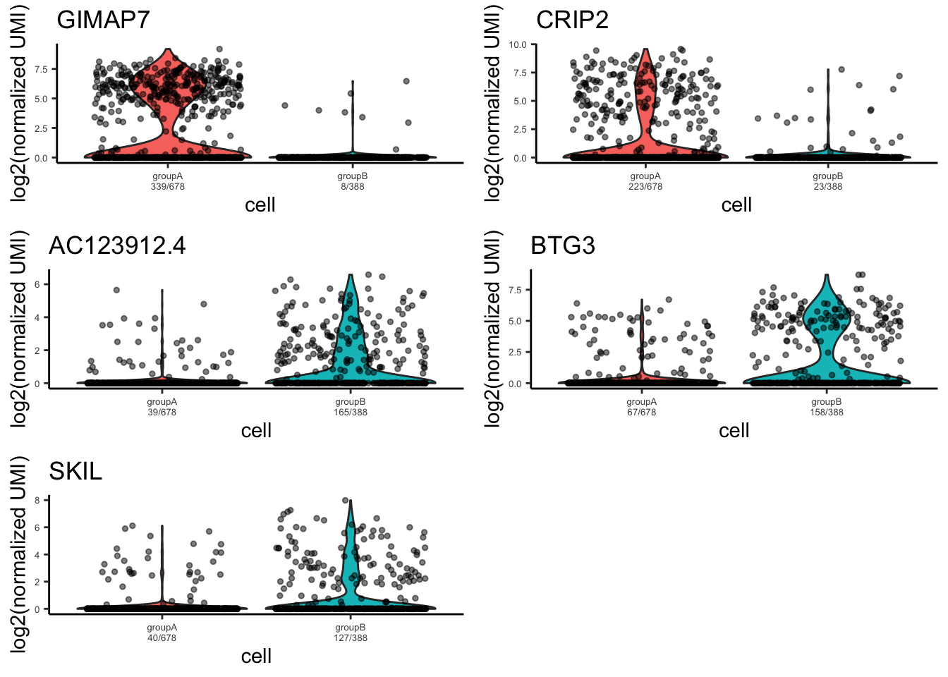
Heatmap for differential genes
plot_heatmap_for_differential_genes(objectA = MPN, objectB = MPN, cellsA = WT_normal.cell_ids, cellsB = WT_patient.cell_ids,
                                    gene_list = rownames(sig.genes))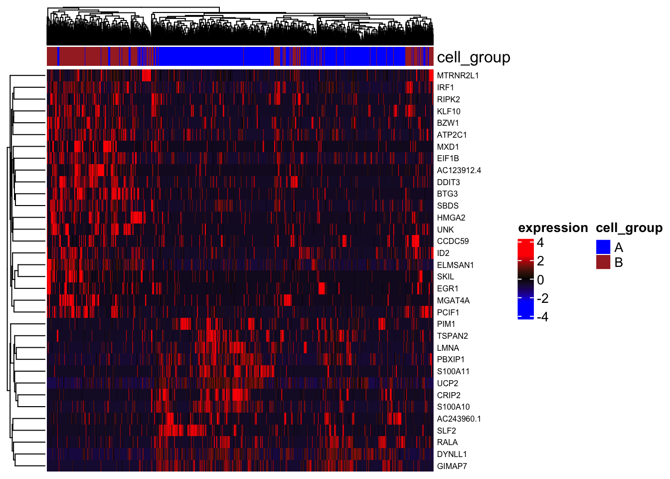
GSEA analysis
First, genes will be pre-ranked.
preranked.genes<-identifyGSEAPrerankedGenes(objectA = MPN, objectB = MPN,
                           cellsA = WT_normal.cell_ids, cellsB = WT_patient.cell_ids)
## [1] "Processing Fisher's exact test!"
## [1] "Processing Wilcoxon Rank-sum test!"
## [1] "Combining p-values using the fisher's method!"Second, fGSEA will be performed with the HALLMARK gene sets.
GSEA.results<-Run_fGSEA_analysis(objectA = MPN, objectB = MPN, eps = 0,
                                 cellsA = WT_normal.cell_ids, cellsB = WT_patient.cell_ids,
                                 GSEAPrerankedGenes_info = preranked.genes,
                                 gmt.file = "../SingCellaR_example_datasets/Human_genesets/h.all.v7.1.symbols.gmt",
                                 plotGSEA = T)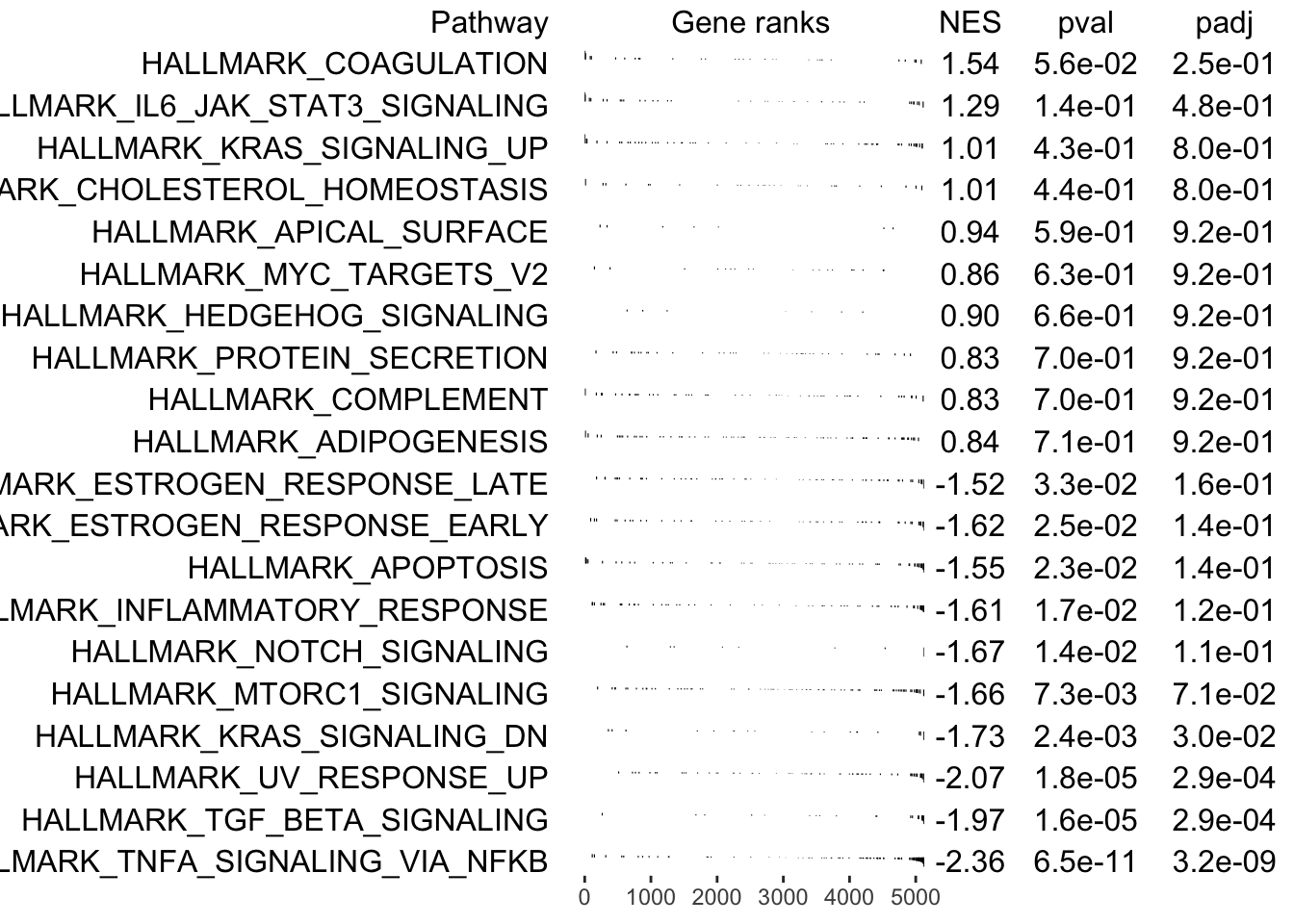
## [1] "Processing GSEA!"Save SingCellaR object for further downstream analyses
save(MPN,file="../SingCellaR_example_datasets/Psaila_et_al/SingCellaR_objects/MPN_v0.1.SingCellaR.rdata")