SingCellaR analysis workflow for 10x Genomics scRNA-seq data
Standard analysis workflow for a myelofibrosis patient (Sample21) generated by Psaila et al., Mol. Cell, 2020
library(SingCellaR)

data_matrices_dir<-"../SingCellaR_example_datasets/Psaila_et_al/Sample21_cellranger/"
Sample21<-new("SingCellaR")
Sample21@dir_path_10x_matrix<-data_matrices_dir
Sample21@sample_uniq_id<-"Sample21"

load_matrices_from_cellranger(Sample21,cellranger.version = 3)
## [1] "The sparse matrix is created."Sample21## An object of class SingCellaR with a matrix of : 33538 genes across 11238 samples.Cell information will be processed. The percentage of mitochondrial per cell will be calculated. For human, mitochondrial gene names start with “MT-”.
process_cells_annotation(Sample21,mito_genes_start_with="MT-")## [1] "List of mitochondrial genes:"
## [1] "MT-ND1" "MT-ND2" "MT-CO1" "MT-CO2" "MT-ATP8" "MT-ATP6" "MT-CO3"
## [8] "MT-ND3" "MT-ND4L" "MT-ND4" "MT-ND5" "MT-ND6" "MT-CYB"
## [1] "The meta data is processed."QC plots
Histogram
plot_cells_annotation(Sample21,type="histogram")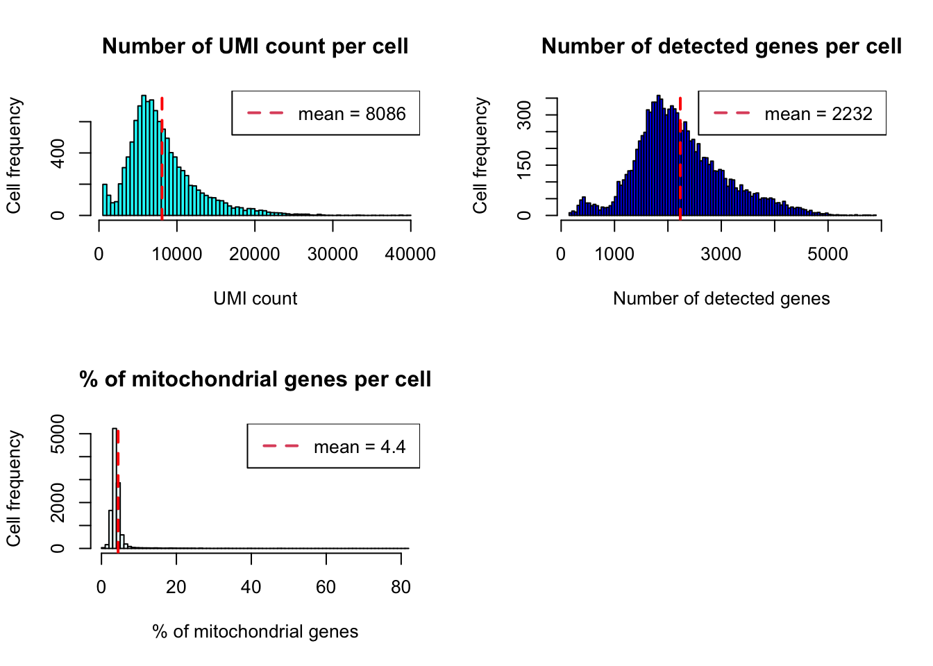
Boxplot
plot_cells_annotation(Sample21,type="boxplot")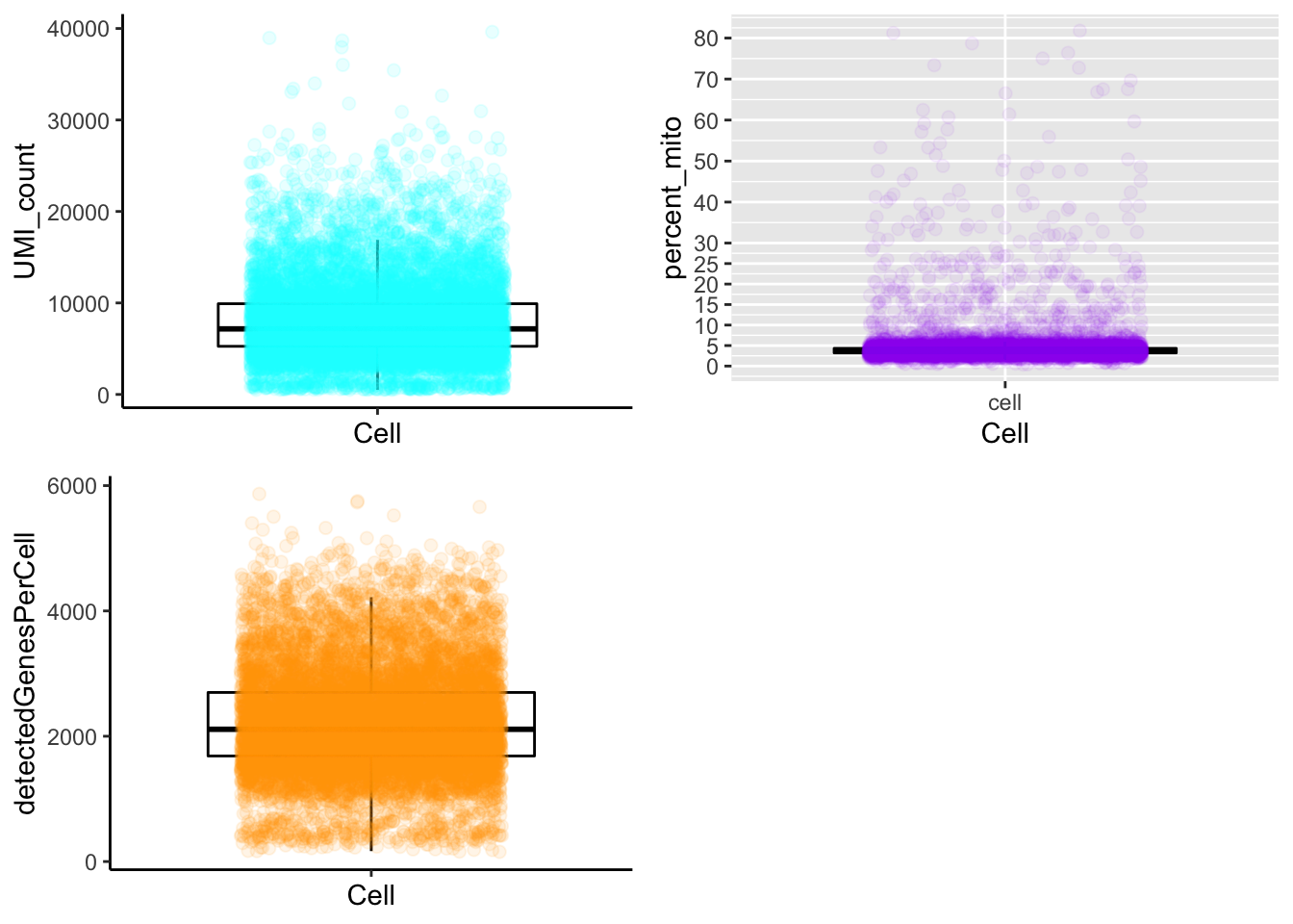
UMI counts/cell vs. number of detected genes/cell
plot_UMIs_vs_Detected_genes(Sample21)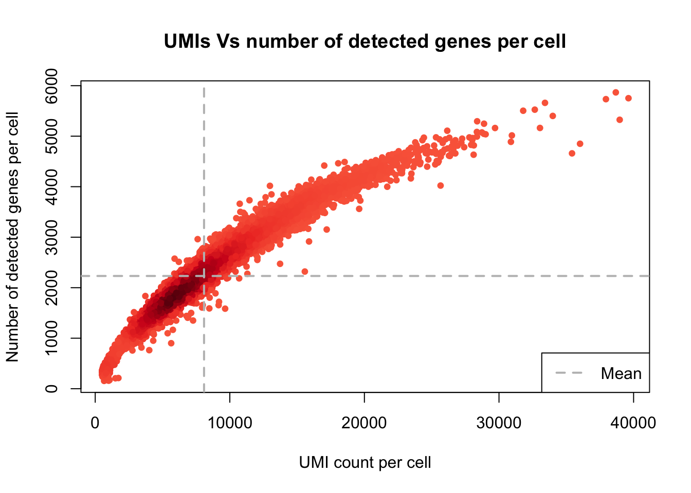
Doublet detection
DoubletDetection_with_scrublet(Sample21)## [1] "Processing Scrublet.."
## [1] "Doublet prediction result is added in the metadata."table(Sample21@meta.data$Scrublet_type)##
## Doublets Singlet
## 1 11237- min_UMIs=1000
- max_UMIs=30000
- min_detected_genes=500
- max_detected_genes=5000
- max_percent_mito=15
- genes_with_expressing_cells=10
Filtering
filter_cells_and_genes(Sample21,
                       min_UMIs=1000,
                       max_UMIs=30000,
                       min_detected_genes=500,
                       max_detected_genes=5000,
                       max_percent_mito=15,
                       genes_with_expressing_cells = 10,
                       isRemovedDoublets = TRUE)
## [1] "The cells and genes metadata are updated by adding the filtering status."
## [1] "362/11238 cells will be filtered out from the downstream analyses!."Normalization
normalize_UMIs(Sample21,use.scaled.factor = T)## [1] "Normalization is completed!."Regressing unwanted source of variations
Next, the effect of the library size and percentage of mitochondrial reads are regressed out.
remove_unwanted_confounders(Sample21,residualModelFormulaStr="~UMI_count+percent_mito")##
|
| | 0%
|
|==== | 6%
|
|======== | 12%
|
|============ | 18%
|
|================ | 24%
|
|===================== | 29%
|
|========================= | 35%
|
|============================= | 41%
|
|================================= | 47%
|
|===================================== | 53%
|
|========================================= | 59%
|
|============================================= | 65%
|
|================================================= | 71%
|
|====================================================== | 76%
|
|========================================================== | 82%
|
|============================================================== | 88%
|
|================================================================== | 94%
|
|======================================================================| 100%
## [1] "Removing unwanted sources of variation is done!"Variable gene detection
get_variable_genes_by_fitting_GLM_model(Sample21,mean_expr_cutoff = 0.05,disp_zscore_cutoff = 0.05)## [1] "Calculate row variance.."
##
|
| | 0%
|
|========= | 12%
|
|================== | 25%
|
|========================== | 38%
|
|=================================== | 50%
|
|============================================ | 62%
|
|==================================================== | 75%
|
|============================================================= | 88%
|
|======================================================================| 100%[1] "Using :12679 genes for fitting the GLM model!"
## [1] "Identified :2129 variable genes"House keeping (e.g., ribosomal genes) and mitochondrial genes should be removed from the list of variable genes. SingCellaR reads in the GMT file that contains ribosomal and mitochondrial genes and removes these genes from the list of highly variable genes. Below shows the example for removing genes.
remove_unwanted_genes_from_variable_gene_set(Sample21,gmt.file = "../SingCellaR_example_datasets/Human_genesets/human.ribosomal-mitocondrial.genes.gmt",
                                             removed_gene_sets=c("Ribosomal_gene","Mitocondrial_gene"))
## [1] "2 genes are removed from the variable gene set."Here, the plot shows highly variable genes in the fitted GLM model.
plot_variable_genes(Sample21)## [1] "Calculate row variance.."
##
|
| | 0%
|
|========= | 12%
|
|================== | 25%
|
|========================== | 38%
|
|=================================== | 50%
|
|============================================ | 62%
|
|==================================================== | 75%
|
|============================================================= | 88%
|
|======================================================================| 100%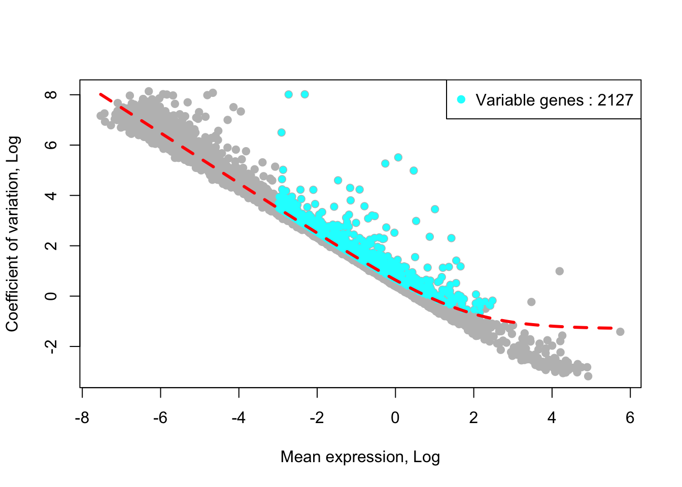
PCA anlysis
Top 50 PCs will be calculated using IRLBA method from https://github.com/bwlewis/irlba The parameter “use.regressout.data” is critical. If TRUE, PCA uses the regressed out data. If FALSE, PCA uses the normalized data without removing unwanted source of variations.
runPCA(Sample21,use.components=50,use.regressout.data = T)## [1] "PCA analysis is done!."Next, the number of PCs used for downstream analyses will be determined from a scree plot.
plot_PCA_Elbowplot(Sample21)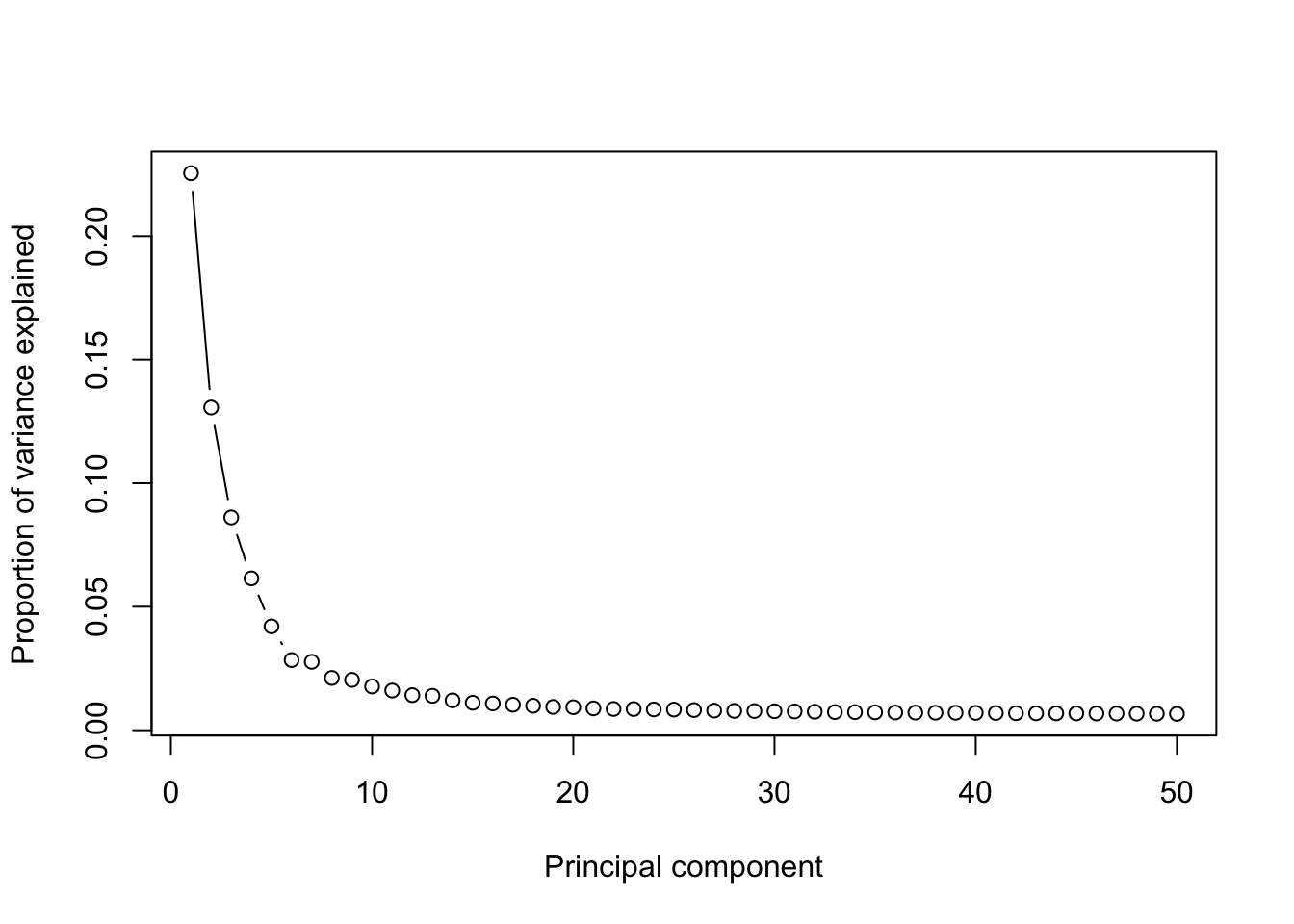
UMAP analysis
runUMAP(Sample21,dim_reduction_method = "pca",n.dims.use = 20,n.neighbors = 30,
        uwot.metric = "euclidean")
## 11:22:30 UMAP embedding parameters a = 1.121 b = 1.057## 11:22:30 Read 10876 rows and found 20 numeric columns## 11:22:30 Using Annoy for neighbor search, n_neighbors = 30## 11:22:31 Building Annoy index with metric = euclidean, n_trees = 50## 0% 10 20 30 40 50 60 70 80 90 100%## [----|----|----|----|----|----|----|----|----|----|## **************************************************|
## 11:22:31 Writing NN index file to temp file /var/folders/c6/_w309xr54n7cphf9nw4x_ms40000gn/T//Rtmp88EKbk/file22d658e45d34
## 11:22:31 Searching Annoy index using 8 threads, search_k = 3000
## 11:22:32 Annoy recall = 100%
## 11:22:32 Commencing smooth kNN distance calibration using 8 threads
## 11:22:33 Initializing from normalized Laplacian + noise
## 11:22:33 Commencing optimization for 200 epochs, with 469086 positive edges
## 11:22:39 Optimization finished## [1] "UMAP analysis is done!."plot_umap_label_by_a_feature_of_interest(Sample21,feature = "UMI_count",point.size = 0.1, mark.feature = FALSE)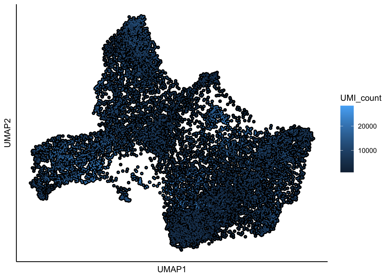
Cluster identification
We further identify clusters using the following function.
identifyClusters(Sample21,n.dims.use = 30,n.neighbors = 30,knn.metric = "euclidean")## [1] "Building Annoy index with metric = euclidean , n_trees = 50"## 0% 10 20 30 40 50 60 70 80 90 100%## [----|----|----|----|----|----|----|----|----|----|## **************************************************|## [1] "Searching Annoy index, search_k = 3000"## 0% 10 20 30 40 50 60 70 80 90 100%
## [----|----|----|----|----|----|----|----|----|----|
## **************************************************|## [1] "Building graph network.."
## [1] "Building graph network is done."
## [1] "Process community detection.."
## [1] "Louvain analysis is done!."Identified clusters are then superimposed on top of the UMAP.
plot_umap_label_by_clusters(Sample21,show_method = "louvain",point.size = 0.80)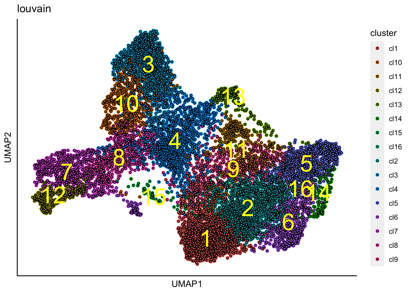
Force-directed graph analysis
SingCellaR incorporates Force-directed graph for the visualization of cell differentiation trajectories.
runFA2_ForceDirectedGraph(Sample21,n.dims.use = 20,
                          n.neighbors = 5,n.seed = 1,fa2_n_iter = 1000)
## [1] "Building Annoy index with metric = euclidean , n_trees = 50"## 0% 10 20 30 40 50 60 70 80 90 100%## [----|----|----|----|----|----|----|----|----|----|## **************************************************|## [1] "Searching Annoy index, search_k = 500"## 0% 10 20 30 40 50 60 70 80 90 100%
## [----|----|----|----|----|----|----|----|----|----|
## **************************************************|## [1] "Processing fa2.."
## [1] "Force directed graph analysis is done!."Force-directed graph is then plotted with identified clusters.
plot_forceDirectedGraph_label_by_clusters(Sample21,show_method = "louvain",vertex.size = 0.85,
                                          background.color = "black")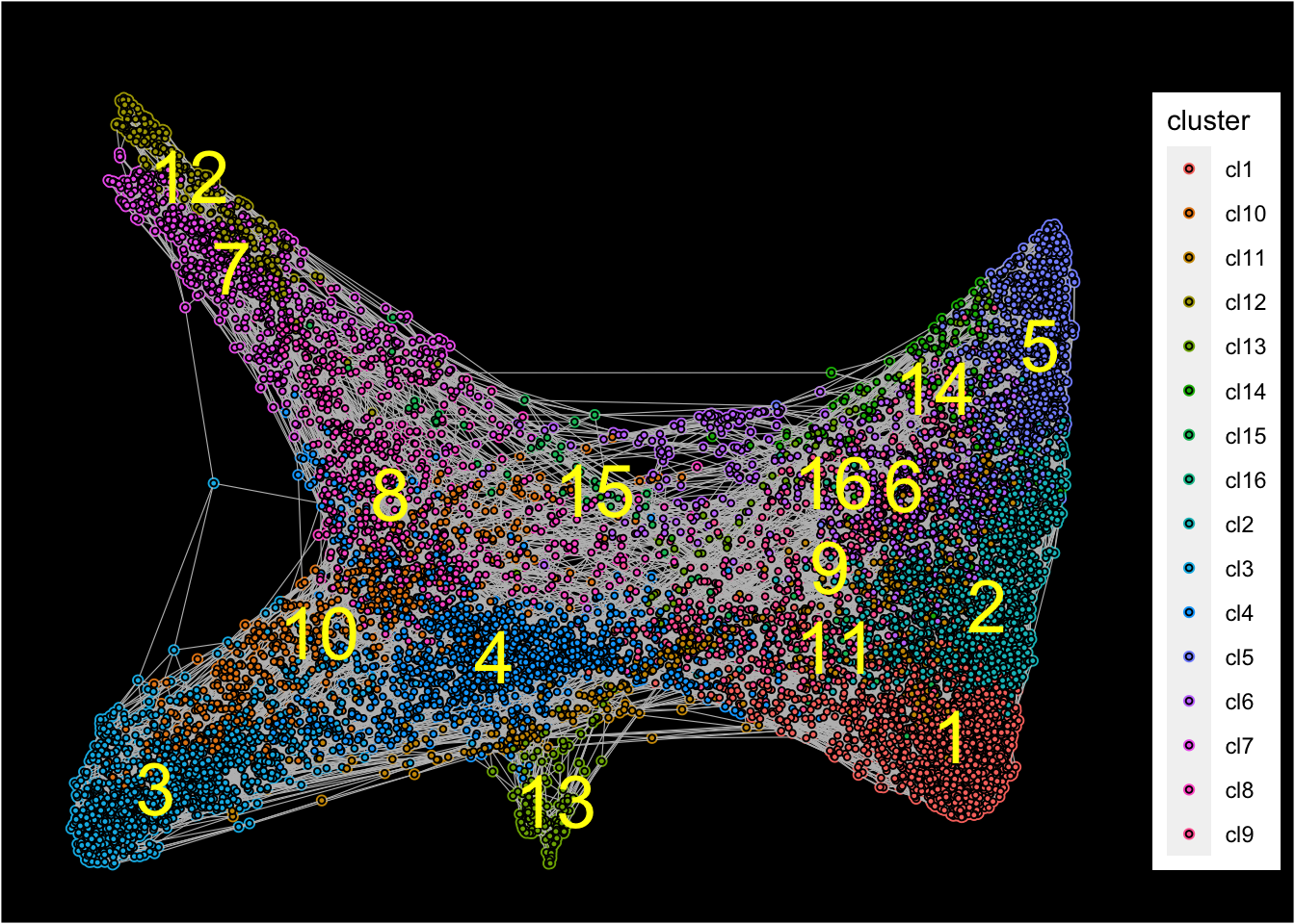
The superimposition of signature gene scores
SingCellaR can superimpose signature gene scores from different gene sets on top of embeddings.
The plots below show the superimposition of gene scores from erythroid, myeloid, lymphoid, and megakaryocytic gene sets on top UMAP and force-directed graph respectively.
plot_umap_label_by_multiple_gene_sets(Sample21,gmt.file = "../SingCellaR_example_datasets/Human_genesets/human.signature.genes.v1.gmt",
                                      show_gene_sets = c("Erythroid","Lymphoid","Myeloid","Megakaryocyte"),
                                      custom_color = c("red","orange","cyan","purple"),
                                      isNormalizedByHouseKeeping = T,point.size = 1,background.color = "black")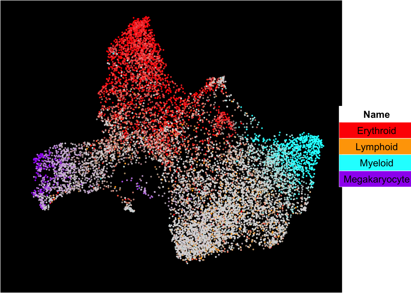
plot_forceDirectedGraph_label_by_multiple_gene_sets(Sample21,gmt.file = "../SingCellaR_example_datasets/Human_genesets/human.signature.genes.v1.gmt",
                                      show_gene_sets = c("Erythroid","Lymphoid","Myeloid","Megakaryocyte"),
                                      custom_color = c("red","orange","cyan","purple"),
                                      isNormalizedByHouseKeeping = T,vertex.size = 1,edge.size = 0.1,
                                      background.color = "black")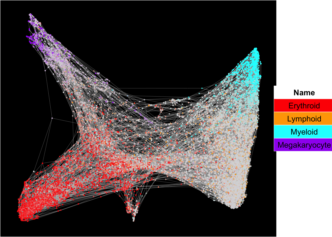
Marker gene identification
Next, we perform differential gene expression analysis across clusters to identify marker genes that are highly expressed in each cluster.
* This step is critical, prepared for the “supervised harmony” integration. Supervised harmony requires differential genes across identified clusters per each sample.
findMarkerGenes(Sample21,cluster.type = "louvain")## [1] "Number of genes for analysis: 15991"
## [1] "Creating binary matrix.."
## [1] "Finding differential genes.."
## [1] "Identifying marker genes for: cl1"
## [1] "Processing Fisher's exact test!"
## [1] "Processing Wilcoxon Rank-sum test!"
## [1] "Combining p-values using the fisher's method!"
## [1] "Identifying marker genes for: cl2"
## [1] "Processing Fisher's exact test!"
## [1] "Processing Wilcoxon Rank-sum test!"
## [1] "Combining p-values using the fisher's method!"
## [1] "Identifying marker genes for: cl3"
## [1] "Processing Fisher's exact test!"
## [1] "Processing Wilcoxon Rank-sum test!"
## [1] "Combining p-values using the fisher's method!"
## [1] "Identifying marker genes for: cl4"
## [1] "Processing Fisher's exact test!"
## [1] "Processing Wilcoxon Rank-sum test!"
## [1] "Combining p-values using the fisher's method!"
## [1] "Identifying marker genes for: cl5"
## [1] "Processing Fisher's exact test!"
## [1] "Processing Wilcoxon Rank-sum test!"
## [1] "Combining p-values using the fisher's method!"
## [1] "Identifying marker genes for: cl6"
## [1] "Processing Fisher's exact test!"
## [1] "Processing Wilcoxon Rank-sum test!"
## [1] "Combining p-values using the fisher's method!"
## [1] "Identifying marker genes for: cl7"
## [1] "Processing Fisher's exact test!"
## [1] "Processing Wilcoxon Rank-sum test!"
## [1] "Combining p-values using the fisher's method!"
## [1] "Identifying marker genes for: cl8"
## [1] "Processing Fisher's exact test!"
## [1] "Processing Wilcoxon Rank-sum test!"
## [1] "Combining p-values using the fisher's method!"
## [1] "Identifying marker genes for: cl9"
## [1] "Processing Fisher's exact test!"
## [1] "Processing Wilcoxon Rank-sum test!"
## [1] "Combining p-values using the fisher's method!"
## [1] "Identifying marker genes for: cl10"
## [1] "Processing Fisher's exact test!"
## [1] "Processing Wilcoxon Rank-sum test!"
## [1] "Combining p-values using the fisher's method!"
## [1] "Identifying marker genes for: cl11"
## [1] "Processing Fisher's exact test!"
## [1] "Processing Wilcoxon Rank-sum test!"
## [1] "Combining p-values using the fisher's method!"
## [1] "Identifying marker genes for: cl12"
## [1] "Processing Fisher's exact test!"
## [1] "Processing Wilcoxon Rank-sum test!"
## [1] "Combining p-values using the fisher's method!"
## [1] "Identifying marker genes for: cl13"
## [1] "Processing Fisher's exact test!"
## [1] "Processing Wilcoxon Rank-sum test!"
## [1] "Combining p-values using the fisher's method!"
## [1] "Identifying marker genes for: cl14"
## [1] "Processing Fisher's exact test!"
## [1] "Processing Wilcoxon Rank-sum test!"
## [1] "Combining p-values using the fisher's method!"
## [1] "Identifying marker genes for: cl15"
## [1] "Processing Fisher's exact test!"
## [1] "Processing Wilcoxon Rank-sum test!"
## [1] "Combining p-values using the fisher's method!"
## [1] "Identifying marker genes for: cl16"
## [1] "Processing Fisher's exact test!"
## [1] "Processing Wilcoxon Rank-sum test!"
## [1] "Combining p-values using the fisher's method!"The heatmap of top 10 genes
plot_heatmap_for_marker_genes(Sample21,cluster.type = "louvain",n.TopGenes = 10,rowFont.size = 5)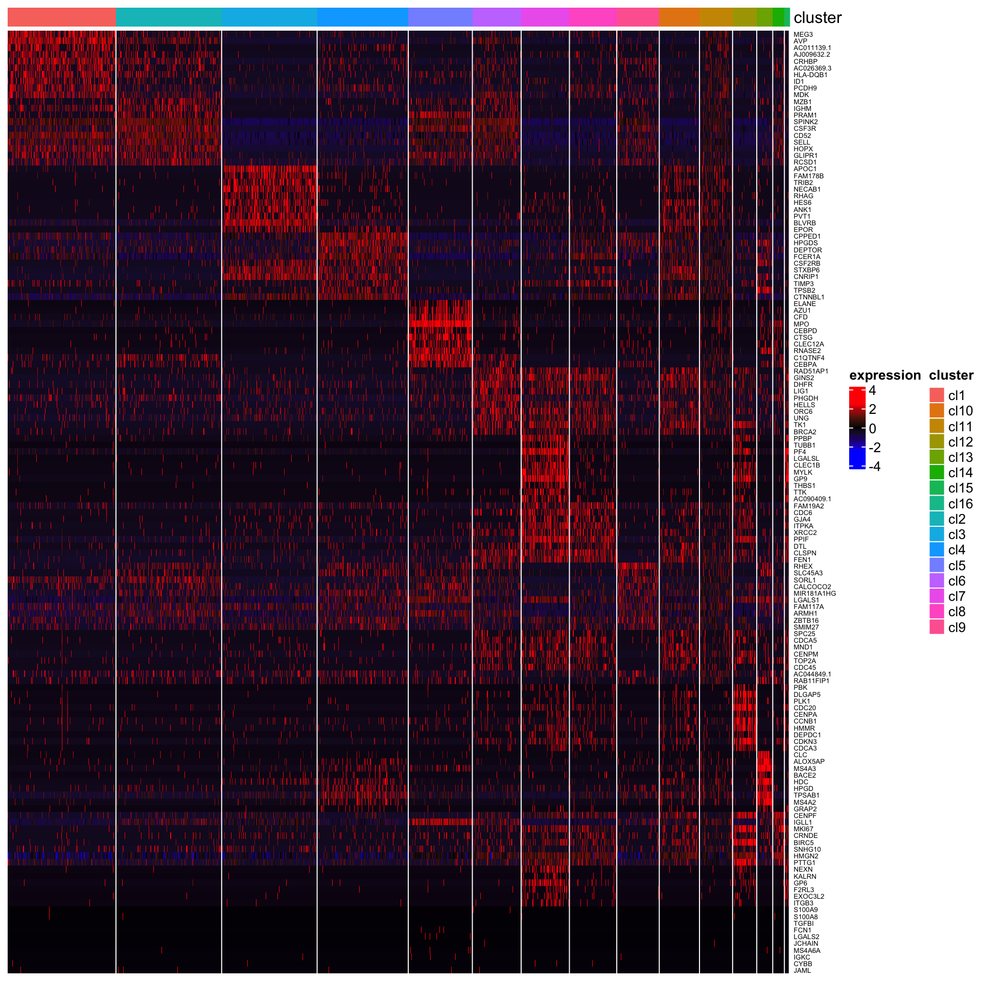
Save SingCellaR object for the integration
Sample21 SingCellaR object will be saved for the integration with other samples.
save(Sample21,file="../SingCellaR_example_datasets/Psaila_et_al/SingCellaR_objects/Sample21.SingCellaR.rdata")